|
MATLAB
RESOURCES INTRODUCTION
TO QUANTUM MECHANICS
3rd
Edition
David
J Griffiths & Darrel F Schroeter
Ian
Cooper matlabvisualphysics@gmail.com CHAPTER 2 THE SCHRODINGER EQUATION DOWNLOAD DIRECTORY FOR MATLAB SCRIPTS simpson1d.m QMG2box.m The starting point for studying
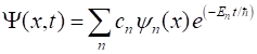
quantum mechanics is the Schrodinger equation. The time dependent [1D]
Schrodinger equation is
The Hamiltonian
operator is
where m is the
mass of the particle and If the
wavefunction
then you
get the time independent Schrodinger equation
where E is the
total energy of the system and The time
independent wavefunction
When
systems are described by such an eigenfunction The
Schrodinger equation is linear. Therefore, the separable solutions are stationary states, in the sense that all
probabilities and expectation values are independent of time, but this property
is emphatically not shared by the general solution when the energies are
different, for different stationary states, and the exponential terms do not
cancel, when you construct When a
system is not is a stationary state, the wavefunction is represented by a sum
of eigenfunctions like those above. In this situation, the oscillatory time
dependence does not cancel out in calculations, but rather accounts for the
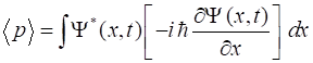
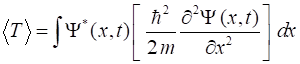
time dependence of physical observables. OPERATORS Physical quantities in quantum mechanics
are calculated via an operator acting upon the wavefunction to give an expectation
value. For [1D] cases: Probability, prob: operator Position,
Momentum,
Kinetic energy, Potential
energy, V Total energy, E A goal
in quantum mechanics is to find solutions of the Schrodinger equation to find
the wavefunction and the total energy
E for a
specified potential energy function PARTICLE
IN A BOX Real
quantum mechanical systems are usually mathematically quite complicated.
However, the so-called particle in a box model can be used to illustrate many of the important
mathematical concepts of quantum mechanics. Although it is an artificial
system, there are many wide-ranging analogies to real systems. This particle
in a box model is instructive as it shows how the quantum mechanical
formalism works in an example that is sufficiently simple to carry out the
calculations step by step. Furthermore, the implications of the symmetry of
the wavefunctions can be seen and the concept of transition from one
stationary state to another can be demonstrated using the Matlab Script QMG2box.m where the
time evolution of the wavefunctions can be animated. I will
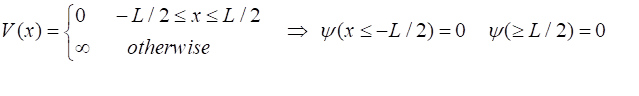
consider the example of an electron confined to a [1D] potential well of
width L where
the potential energy function
So, in
the region
This
model is called the particle in a box model.
It is very easy to solve the Schrodinger equation for the particle in a box
model. The are infinite number of stationary state solutions given by the
quantum number N where N = 1, 2,
3, … . The
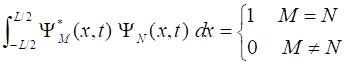
normalized stationary state wavefunctions are
where The
stationary wavefunctions form an orthonormal
vector space where
The
eigenvalues for the energy levels are The
total energy E of the
system is quantized. The energy does
not vary continuously but is proportional to the square of the quantum number
N. Zero
total energy is not permitted – the total energy of the particle in the
box is always greater than zero. The lowest energy state is called the zero-point energy state or ground-state
energy
In this ideal case of an electron
trapped in a box, it is not so different than an electron bound to the
nucleus of an atom. If the
width of the box is in the order of nanometres, the energies for the electron
in the box are of the same order of magnitude as actual atomic energy levels.
If you replace the electron by a proton in a box of width in the order of
femtometres, the energies are millions of times greater, which gives a clue
to why nuclear fission or fusion reactions have energy scales millions of
times greater than in chemical reactions. Using a
Matlab Script, you can explore the bound electron in the box in much greater
depth than is possible by a presentation of the content in a textbook. I will
consider two stationary states given by the integers M and N and the
non-stationary state that is a linear combination of the two stationary
states in the Script QMG2box.m
If you
want to examine a single stationary state, then set M = N. QMG2box.m Inputs: M N
quantum numbers cM cN
coefficients for compound wavefunction (unnormalized) L
width of potential well numX
number of spatial grid points numT
number of time grid points Computations: EM EN
total energies wM wN fM fN PM PN
angular frequencies, frequencies, periods psiM psiN spatial wavefunctions PSIM PSIN stationary state
wavefunctions pdM
pdN
probability densities xAVG EAVG expectation
values: position and total energy HX HP
Fourier transforms: position <x> and energy at a fixed x position Example
1 Quantum
numbers, M = 2 N =
3 Check
normalization: normM = 1.0000 normN
= 1.0000 normMN
= 1.0000 Orthonormal
= 0.0000 STATIONARY
STATES M and N Total energies: EM = 6.0165 eV EN = 13.5371 eV Ang. frequencies omegaM
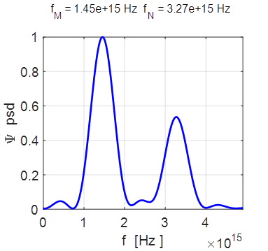
= 9.14e+15 rad/s omegaN = 2.06e+16 rad/s Frequencies fM
= 1.45e+15 Hz fN = 3.27e+15 Hz Periods PM = 0.69 fs PN =
0.31 fs COMPOUND
STATE MN coeff: cM^2
= 0.0588 cN^2
= 0.9412 cM^2+cN^2 = 1.0000 Total energy <EMN>
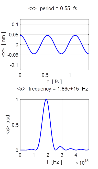
= 13.0904 eV <x> period = 0.5471 fs <x> frequency = 1.8608e+15
Hz Dipole radiation dE = 7.5206 eV
The two
stationary states have different symmetries and as a result, the compound
wavefunction sloshes backward and forwards.
Fourier transform of the compound state
showing the power spectral density (psd).
The time evolution of the expectation value
for position, <x> and its power density spectrum. The
expectation value of position oscillates with simple harmonic motion when
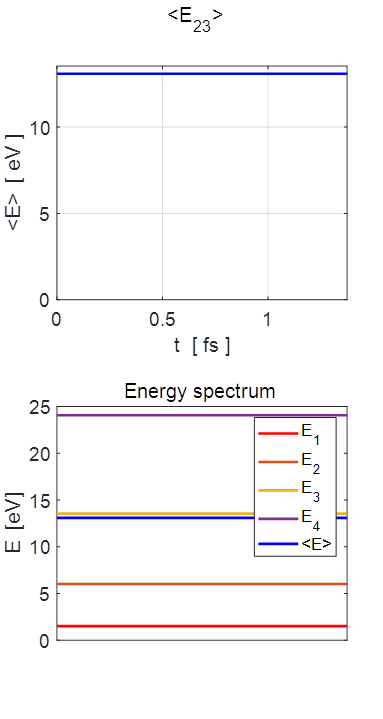
The energy spectrum for the particle in a
box model and the expectation value for the total energy <E> = 13.0904 eV. The expectation value for the energy agrees
with the prediction The expectation value <E> is
time independent. Selection
rules The
particle in a box model may be used to study transitions between stationary
states, induced by electromagnetic radiation. A transition from a higher
energy level stationary state to one with lower energy can be attributed to
the radiation of an electric dipole. The transition and radiation between stationary
states is determined by the change in quantum number
If In this
example dn = 1, so dipole radiation can
occur and the energy of the photon emitted is 7.5206
eV = When one of the quantum numbers is odd the
other even, the probability density sloshes backwards and forwards about the
centre of the potential well at x = 0 and the expectation value <x> oscillates around x = 0 executing simple harmonic
motion. The expectation value for position oscillates sinusoidally, at an
angular frequency
T = 0.55 fs f = 1.86x10¹⁵ Hz Example
2 Quantum
numbers, M = 2 N =
4 Check
normalization: normM = 1.0000 normN
= 1.0000 normMN
= 1.0000 Orthonormal
= 0.0000 STATIONARY
STATES M and N Total energies: EM = 6.0165 eV EN = 24.0659 eV Ang. frequencies omegaM
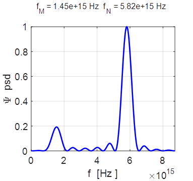
= 9.14e+15 rad/s omegaN = 3.66e+16 rad/s Frequencies fM
= 1.45e+15 Hz fN = 5.82e+15 Hz Periods PM = 0.69 fs PN =
0.17 fs COMPOUND
STATE MN coeff: cM^2
= 0.2000 cN^2
= 0.8000 cM^2+cN^2 = 1.0000 Total energy <EMN>
= 20.4445 eV <x> = 0 Dipole radiation forbidden
The two
stationary states have the same symmetries and as a result, the compound
wavefunction is symmetrical about x = 0, so no electric dipole can be created
as <x> = 0 at all times. In this example dn
= 2, an even number, so dipole radiation cannot occur.
Fourier transform of the compound state
showing the power spectral density (psd).
The energy spectrum for the particle in a
box model and the expectation value for the total energy <E>
= 20.445
eV. The expectation value for the energy agrees
with the prediction The expectation value <E> is
time independent.
|