|
MATLAB
RESOURCES FOR INTRODUCTION
TO QUANTUM MECHANICS
3rd
Edition
David
J Griffiths & Darrel F Schroeter
Ian
Cooper matlabvisualphysics@gmail.com CHAPTER 1 THE WAVE FUNCTION STATISTICAL INTERPRETATION PROBABILITY DOWNLOAD DIRECTORY FOR MATLAB SCRIPTS simpson1d.m calculate
the definite integral a function QMG1A.m QMG1B.m QMG1C.m QMG1D.m QMG1E.m QMG1G.m QMG1H.m QMG1J.m QMG1K Probability:
discrete variables Probability plays a central role in quantum mechanics because of the
statistical interpretation that is necessary to predict the outcome of an
experiment. I will consider a simple example of a room filled with people of
different ages. Through this example, we can introduce some terminology and
notation that is essential in understanding quantum mechanics. All the
calculations of the necessary quantities and computed using Matlab. A distribution is setup for the people in the room with ages from 10 to
22. The variables are j ages
from 10 to 22 Nj number
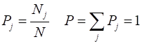
of people of age j N total
number of people in room Pj probability
of person being of age j P total
probability P = 1 <j> average
age jmax most
probable age jmedian median
age <j2> average
of j2 Relationships The
Script QMG1A.m is used to setup the distribution and compute all of the
above variables. In
quantum mechanics the mean or average value is called an expectation value. The standard deviation is a measure of the
spread of the distribution. |

|
QMG1A.m clear;
close all; clc %
PROBABILITY: PEOPLE IN A ROOM % j age of people from 10 to 22 j = 10:22; j = j'; % L number of ages L = length(j); %
Nj number of people aged j:
distribution function Nj = round( 50.*exp(-(18-j).^2./5)
+ 3.*randn(L,1) ); Nj(Nj < 0)
= 0; % N
total number of people N = sum(Nj); % P Probability of person of age j Pj = Nj/ N; % P Probability
of all ages P = sum(Pj); %
Pmax Most probable age ind = find(Pj == max(Pj)); jMax = j(ind); % avgAge
average (mean) age jAvg =
sum(j.*Pj) ; % medianAge
median age cumS = cumsum(Nj); ind = find(cumS > N/2,1); jMedian = j(ind)-1; % avgSq
average of the squares j2Avg = sum(j.^2.*Pj); %
variance and standard deviation (sigma) variance = j2Avg - jAvg^2; sigma = sqrt(variance); %
DISPLAY fprintf('\n Total number of people, N = %2.0f \n',N); table(j, Nj,Pj) fprintf('\n Average age, jAvg =
%2.0f \n',jAvg); fprintf('\n Most probable age, jMax =
%2.0f \n',jMax); fprintf('\n Median age, jAvg =
%2.0f \n',jMedian); fprintf('\n Average of the squares of the ages, j2Avg =
%2.3f \n',j2Avg); fprintf('\n Variance = jAvg =
%2.3f \n',variance); fprintf('\n standard deviation, sigma = %2.3f \n',sigma); %
GRAPHICS figure(1) pos = [0.02 0.05 0.25 0.25]; set(gcf,'Units','normalized'); set(gcf,'Position',pos); set(gcf,'color','w'); bar(j',Nj') xlabel('age j') ylabel('N_j') set(gca,'fontsize',14)
Total
number of people, N = 192 j Nj Pj
10 2 0.010417 11 0
0 12 1 0.0052083 13 0
0 14 5 0.026042 15 5 0.026042 16 19 0.098958 17 39 0.20312 18 41 0.21354 19 45 0.23438 20 23 0.11979 21 6 0.03125 22 6 0.03125 Average age, jAvg
= 18 Most probable age, jMax
= 19 Median age, jAvg
= 17 Average of the squares of the ages,
j2Avg = 327.411 Variance = jAvg
= 3.599 standard deviation, sigma = 1.897 The
figure shown below has a larger value of its standard deviation than the bar
graph shown above.
|


|
QMG Problem 1.10 Consider the first 25 digits of the number ·
Selecting
a digit at random, calculate the probability of getting a 0, 1, 2, … , 9. ·
Draw
a histogram that shows the frequency of each digit. Find ·
most
probable digit? ·
median
digit? ·
average
value? ·
standard
deviation for this distribution |
|
QMG1G.m clear;
close all;clc % SETUP PI = '3141592653589793238462643'; L = length(PI); N = zeros(10,1); PIs = sort(PI); %
Frequency of each digit for c = 1:10 N(c) = count(PI,num2str(c-1)); end %
Probabilities prob = N./25; %
Expectation values c = 1:9; r = N(2:end)'; cavg =
sum(c.*r)/L; c2avg = sum(c.^2.*r)/L; sigma = sqrt(c2avg
- cavg^2); % OUTPUT
disp(PI) disp(PIs) fprintf('Median value = %2.0f \n', str2double(PIs(12))) fprintf('Most common value = %2.0f \n', c(N == max(N))-1) fprintf('Average value = %2.4f \n', cavg) fprintf('standard deviation = %2.4f \n', sigma) ct = 0:9; ct = ct'; table(ct,N,prob) %
GRAPHICS figure(1) x = 0:9; bar(x,N,'b') xlabel('c') ylabel('N(c)') set(gca,'fontsize',14) >>
3141592653589793238462643 1122233333444555666788999 Median
value = 4 Most
common value =
3 Average
value = 4.7200 standard
deviation = 2.4742 ct N prob 0 0 0 1 2 0.08 2 3 0.12 3 5 0.2 4 3 0.12 5 3 0.12 6 3 0.12 7 1 0.04 8 2 0.08 9 3 0.12 |

|
Probability:
continuous variables Consider the continuous variable x defined in the interval from where If our interval extends from -
expectation
value of the function QMG Example 1.2 / Problem 1.2 Suppose someone
drops a rock off a cliff of height h. As it falls, a million photographs are snapped at random intervals.
On each picture the distance the rock has fallen is measured. What is the average
of all these distances (the time average of the distance travelled)?
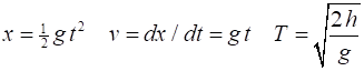
The
distance x fallen
by the rock in time t, the
velocity v and
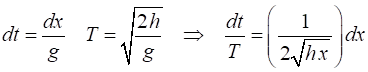
time of flight T are The probability
that a particular photo was taken in the interval t to t + dt
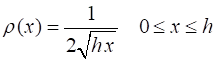
is dt/T Therefore,
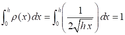
the probability density is So, the
probability of a measure for 0 to h must be 1 The average
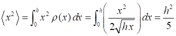
distance (expectation value) is The average
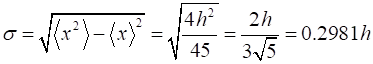
square of the distance is The standard
deviation is The rock starts out
at rest, and picks up speed as it falls; it spends more time near the top, so
the average distance will surely be less than h/2 > h/3. What is the
probability that a photograph, selected at random, would show a distance x more than one standard deviation away from the average? The above
integrals do not have to be evaluated by hand. A much more efficient way is
to use the symbolic tools available in Matlab. All unknown quantities can be
evaluated within a Matlab Script.
But in Matlab, you can do more than this. We can actually stimulate
the taking of the one million snapshoots. |

|
QMG1B.m clear;close all;clc % SETUP h = 1; g = 9.8; nT = 1e6; T = sqrt(2/g); % time of flight t = T.*rand(nT,1); % time x = 0.5*g.*t.^2; % height measurement xavg = mean(x); % <x> expectation value xstd = std(x); % sigma standard deviation %
Probability <x> - sigma <= x <= <x> + sigma ind1 = find(sort(x) > xavg-xstd,1); ind2 = find(sort(x) > xavg+xstd,1); prob1 = (ind2-ind1)/nT; %
Probability x < <x> - sigma and x > <x> + sigma prob2 = 1 - prob1; % OUTPUT fprintf('time of flight, T = %2.4f \n', T) fprintf('expectation value, <x> = %2.4f \n', xavg) fprintf('standard deviation of x, std = %2.4f \n', xstd) fprintf('Probability <x> - sigma <= x <= <x> +
sigma, prob1 = %2.4f \n', prob1) fprintf('Probability x
< <x> - sigma and x > <x> + sigma , prob2 = %2.4f \n', prob2) % GRAPHICS figure(1) pos = [0.52 0.05 0.27 0.27]; set(gcf,'Units','normalized'); set(gcf,'Position',pos); set(gcf,'color','w'); plot(t,x,'.') xlabel('t') ylabel('x') set(gca,'FontSize',12) grid on
time of
flight, T = 0.4518 expectation
value, <x> = 0.3336 standard
deviation of x, std = 0.2981 Probability
<x> - sigma <= x <= <x> + sigma, prob1 = 0.6072 Probability
x < <x> - sigma and x > <x> + sigma ,
prob2 = 0.3928 You can
run the program multiple times and with different numbers of snapshoots to
see how the expectation value <x> changes. nT = 103 0.3200 0.3296 0.3423 nT = 104 0.3315 0.3300 0.3352 nT = 106 0.3336 0.3334 0.3331 You can
also use the symbolic toolbox to perform the necessary integrations. clear;close all;clc syms x h %
probability density probD =
1/(2*sqrt(h*x)); % probabilty symbolic
Ps = int(probD,x); % Probability P = int(probD,x,[0 h]); fprintf('Probability 0<= x <= 1), P = %2.4f \n',P) % Expection value for position <x> xProbD = x*probD; xavg = int(xProbD,x,[0 h]); disp(' ') displayFormula(" xAVG = xavg") % Standard
deviation h
= 1 x2avg = int(x^2*probD,[0
h]); displayFormula("x2AVG = x2avg") xavg2 = xavg^2; displayFormula("xAVG2 = xavg2") sigma2 = x2avg - xavg2; displayFormula("variance = sigma2") sigma = sqrt(sigma2); displayFormula(" STD = sigma") fprintf('STD/h = %2.4f \n',subs(sigma,1)) disp(' ') % Prob
within 1 STD of mean %L1 = subs(xavg -xSTD,1); L2 = subs(xavg +
xSTD,1); L1 = subs(xavg - sigma,1); L2 = subs(xavg
+ sigma,1); Psigma = (int(probD,[L1 L2])); disp('Prob <x> - sigma <= x <= <x> + sigma') fprintf(' Psigma = %2.4f \n',subs(Psigma,1)) disp('Prob x < <x> - sigma or x > <x> +
sigma') fprintf(' 1 - Psigma = %2.4f \n',1 - subs(Psigma,1)) >> Probability
0<= x <= 1), P = 1.0000 xAVG == h/3 x2AVG ==
h^2/5 xAVG2 ==
h^2/9 variance
== (4*h^2)/45 STD ==
((4*h^2)/45)^(1/2) STD/h =
0.2981 Prob
<x> - sigma <= x <= <x> + sigma Psigma =
0.6071 Prob x
< <x> - sigma or x > <x> + sigma 1 - Psigma =
0.3929 |

|
QMG
Problem
1.3 Gaussian distribution Consider
the Gaussian function for the probability density
Determine
I could
not integral the probability density symbolically. However, the problem can
be done using numerical methods, i.e., numerical values need to be assigned
for A, k, x and the
limits for the integration. The
normalized Gaussian function for the probability density is So,
given a value for k, we can
check the normalized value for A, the
standard deviation |

|
QMGC.m simpson1d.m clear;
close all; clc % SETUP:
Gaussian function - probability density, rho % Peak
value A = 1; % Decay
constant k = 2; % Limits
x L1 = -2; L2 = 4; % Centre
of Gaussian function a = 1; % x
values N = 9999; x = linspace(L1,L2,N); %
Probability density, rho rho = A.*exp(-k.*(x-a).^2); %
Normalize probability density AN = simpson1d(rho,L1,L2); A = A/AN; %
Gaussian function: probability density, rho rho = A.*exp(-k.*(x-a).^2); check = simpson1d(rho,L1,L2); %
Expectation value <x>, xavg fn = x.*rho; xavg =
simpson1d(fn,L1,L2); %
Expectation value <x^2>, x2avg fn = x.^2.*rho; x2avg = simpson1d(fn,L1,L2); %
Standard deviation, sigma sigma = sqrt(x2avg
- xavg^2); % Theoretical
predictions AT = 1/(sigma*sqrt(2*pi)); kT =
1/(2*sigma^2); xavgT = a; % OUTPUT fprintf('Check normalization: prob = %2.4f \n', check) fprintf('normalized amplitude, A = %2.4f \n', A) fprintf('THEORY: normalized amplitude, A = %2.4f \n', AT) fprintf('decay constant, k = %2.4f \n', k) fprintf('THEORY: decay constant, k = %2.4f \n', kT) fprintf('expectation value, <x> = %2.4f \n', xavg) fprintf('THEORY: expectation value, <x> = %2.4f \n', xavgT) fprintf('expectation value, <x^2> = %2.4f \n', x2avg) fprintf('Standard deviation, sigma = %2.4f \n', sigma) %
GRAPHICS figure(1) set(gcf,'units','normalized'); set(gcf,'position',[0.35 0.05 0.25 0.25]); set(gcf,'color','w'); FS = 14; plot(x,rho,'b','LineWidth',2) xticks([L1:1:L2]) grid on xlabel('x') ylabel('\rho') set(gca,'FontSize',FS)
Check
normalization: prob = 1.0000 normalized
amplitude, A = 0.7979 THEORY:
normalized amplitude, A = 0.7979 decay
constant, k = 2.0000 THEORY:
decay constant, k = 2.0000 expectation
value, <x> = 1.0000 THEORY:
expectation value, <x> = 1.0000
expectation
value, <x^2> = 1.2500 Standard
deviation, sigma = 0.5000 |

|
Normalization In a
[1D] system, a particle is quantum mechanics is described by a wavefunction Since
the particle must be somewhere and the
wavefunction is said to be normalized.
If the wavefunction is normalized at t = 0, then
it stays normalized for all future time. Physically realizable states given
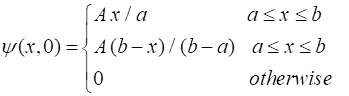
by the wavefunction QMG Problem 1.4 At time t
= 0 a particle is represented by the
wavefunction where A, a, and b are
positive constants. Normalize
the wavefunction. Where is
the particle most likely to be found? What is
the probability of finding the particle to the left of a? What
is the expectation <x>? What is
the standard deviation, |
|
QMG1D.m
simpson1d.m We can
answer the above questions using Matlab symbolic functions. Run
cells 1 and 2 separately. %% CELL
1 clear;
close all;clc % SETUP A = 1; a = 2; b = 5; N = 999; x = linspace(0,b,N); psi = (A/a).*x; psi(x>a) = A.*(b-x(x>a))./(b-a); %
Normalize the wavefuntion AN = simpson1d(psi.^2,0,b); psi = psi./sqrt(AN); A = A/sqrt(AN); check = simpson1d(psi.^2,0,b); % Most
likely postion to find the particle xM = x(psi == max(psi)); %
Probability of x < a ind1 = 1;ind2
= find(x>a,1); R = ind1:ind2; % WARNING R must be an odd number L = length(R); if mod(L,2) == 0, ind2
= ind2+1; end R = ind1:ind2; probA =
simpson1d(psi(R).^2,x(ind1),x(ind2)); %
Probability of x > a ind1 = find(x>a,1); ind2 = N; R = ind1:ind2; % WARNING R must be an odd number L = length(R); if mod(L,2) == 0, ind2
= ind2+1; end R = ind1:ind2; probB =
simpson1d(psi(R).^2,x(ind1),x(ind2)); %
Expectation <x> fn = psi.*x.*psi; xavg =
simpson1d(fn,0,b); %
Expectation <x2> fn = psi.*x.^2.*psi; x2avg = simpson1d(fn,0,b); sigma = sqrt(x2avg
- xavg^2); %
Probability of xavg-sigm < x < xavg+sigma ind1 = find(x>xavg-sigma,1);ind2 = find(x>xavg+sigma,1); R = ind1:ind2; % WARNING R must be an odd number L = length(R); if mod(L,2) == 0, ind2
= ind2+1; end R = ind1:ind2; probS =
simpson1d(psi(R).^2,x(ind1),x(ind2)); % OUTPUT fprintf('Check normalization: prob = %2.4f \n', check) fprintf('Normalized amplitude, A = %2.4f \n', A) fprintf('Most likely postion, xM = %2.4f
\n', xM) fprintf('Expectation value, <x> = %2.4f \n', xavg) fprintf('Standard deviation, sigma = %2.4f \n', sigma) fprintf('Probability x < a = %2.4f \n', probA) fprintf('Probability x > a = %2.4f \n', probB) fprintf('Probability x-sigma < x < x+sigma
= %2.4f \n', probS) %
GRAPHICS figure(1) set(gcf,'units','normalized'); set(gcf,'position',[0.35 0.05 0.25 0.35]); set(gcf,'color','w'); FS = 14; subplot(2,1,1) xP = x; yP = psi; plot(xP,yP,'b','LineWidth',2) grid on xlabel('x') ylabel('\psi(x,0)') set(gca,'FontSize',FS) subplot(2,1,2) xP = x; yP = psi.^2; plot(xP,yP,'b','LineWidth',2) hold on area(x(R),psi(R).*psi(R)) grid on xlabel('x') ylabel('|\psi(x,0)|^2') set(gca,'FontSize',FS)
Check
normalization: prob = 1.0000 Normalized
amplitude, A = 0.7746 Most
likely postion, xM =
1.9990 Expectation
value, <x> = 2.2500 Standard
deviation, sigma = 0.7984 Probability
x < a = 0.4024 Probability
x > a = 0.5976 Probability
x-sigma < x < x+sigma = 0.6834 Matlab
Symbolic toolbox %% CELL #2 clear;
close all; clc syms x a b A fn1 =
x/a S1 = int(fn1^2, [0 a]) fn2 =
((b-x)/(b-a)) S2 = int(fn2^2,[a b]) S = S1 +
S2 A =
1/sqrt(S) psi1 =
A*fn1 psi2 =
A*fn2 probA1 =
int(psi1^2,[0 a]) probA2 =
int(psi2^2,[a b]) xavg1 = int(x*psi1^2,[0 a]) xavg2 = int(x*psi2^2,[a b]) xavg = xavg1 + xavg2 >> fn1 =
x/a S1 = a/3 fn2 =-(b - x)/(a - b) S2 = b/3
- a/3 S = b/3 A =
1/(b/3)^(1/2) psi1 =
x/(a*(b/3)^(1/2)) psi2 =
-(b - x)/((a - b)*(b/3)^(1/2)) probA1 =
a/b probA2 =
1 - a/b xavg1 =
(3*a^2)/(4*b) xavg2 =
a/2 + b/4 - (3*a^2)/(4*b) xavg = a/2 + b/4 |

|
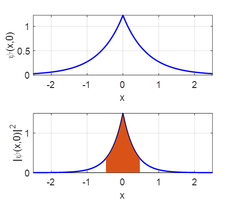
QMG Problem 1.5 Consider the wave
function where A, k, and ω are positive real constants. Normalize the
wavefunction. Determine the
<x> and Probability a
measurement of x is in the range
I will
only consider a numerical approach to the problem where numerical values are
assigned to the constants. You only need to consider the time independent
wavefunction |
|
QMG1E.m
simpson1d.m clear;
close all;clc % SETUP A = 1; k = 1.5; x1 = -2.5; x2 = 2.5; N = 9999; x = linspace(x1,x2,N); psi = A.*exp(-k*abs(x)); % Normalize
the wavefuntion AN = simpson1d(psi.^2,x1,x2); psi = psi./sqrt(AN); A = A/sqrt(AN); check = simpson1d(psi.^2,x1,x2); % Most
likely postion to find the particle xM = x(psi == max(psi)); % %
Probability of x < a % probA
= simpson1d(psi.^2,0,a); % %
Probability of x > a % probB
= simpson1d(psi.^2,a,b); %
Expectation <x> fn = psi.*x.*psi; xavg =
simpson1d(fn,x1,x2); %
Expectation <x2> fn = psi.*x.^2.*psi; x2avg = simpson1d(fn,x1,x2); sigma = sqrt(x2avg
- xavg^2); %
Probability of xavg-sigm < x < xavg+sigma ind1 = find(x>xavg-sigma,1);ind2 = find(x>xavg+sigma,1); R = ind1:ind2; % WARNING R must be an odd number L = length(R); if mod(L,2) == 0, ind2
= ind2+1; end R = ind1:ind2; probS =
simpson1d(psi(R).^2,x(ind1),x(ind2)); % OUTPUT fprintf('Check normalization: prob = %2.4f \n', check) fprintf('Normalized amplitude, A = %2.4f \n', A) fprintf('Most likely postion, xM = %2.4f
\n', xM) fprintf('Expectation value, <x> = %2.4f \n', xavg) fprintf('Standard deviation, sigma = %2.4f \n', sigma) fprintf('Probability x-sigma < x < x+sigma
= %2.4f \n', probS) %
GRAPHICS figure(1) set(gcf,'units','normalized'); set(gcf,'position',[0.35 0.05 0.25 0.35]); set(gcf,'color','w'); FS = 14; subplot(2,1,1) xP = x; yP = psi; plot(xP,yP,'b','LineWidth',2) grid on xlabel('x') ylabel('\psi(x,0)') set(gca,'FontSize',FS) subplot(2,1,2) xP = x; yP = psi.^2; plot(xP,yP,'b','LineWidth',2) hold on area(x(R),psi(R).*psi(R)) grid on xlabel('x') ylabel('|\psi(x,0)|^2') set(gca,'FontSize',FS) >> Check
normalization: prob = 1.0000 Normalized
amplitude, A = 1.2251 Most
likely postion, xM =
0.0000 Expectation
value, <x> = -0.0000 Standard
deviation, sigma = 0.4667 Probability x-sigma
< x < x+sigma = 0.7541 |
|
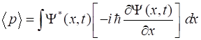
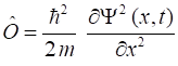
MOMENTUM and THE UNCERTAINTY PRINCIPLE Physical quantities in quantum mechanics
are calculated via an operator acting upon the wavefunction to give an
expectation value. For [1D] cases: Probability, prob: operator Position,
Momentum,
Kinetic energy, Potential
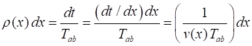
energy, V Total energy, E QMG Problems 1.11 1.12 1.13 Imagine
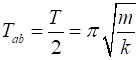
a particle of mass m and energy E in a potential well sliding
frictionlessly back and forth between the classical turning points (a and b).
The velocity of the particle is v(x). Classically, the
probability of finding the particle in the range dx is equal to the
fraction of the time dt it spends in the interval dx to the
time Tab it takes to get from a to b where Find the
expectation (average) position of the particle and its standard deviation for
a simple harmonic oscillator where
Conservation
of energy Time
interval Tab |


|
QMG1H.m clear;
close all;clc % SETUP A = 1; %
amplitude k = 2; %
spring constant m = 2; %
mass E = 0.5*k*A^2; %
total energy N = 99999; %
grid points x1 = -A; x2 = A; %
limits a and b x = linspace(x1,x2,N);
% x position V = 0.5*k*x.^2; %
potential energy v = sqrt(2*(E-V)/m); % velocity Tab = pi*sqrt(m/k); % time interval a to
b rho = 1./(v.*Tab); %
probability density %
POSITION: Probabilities / expectation values / standard deviation Xrho =
x.*rho; R = 2:N-1;
% v --> then rho --> infinity fn = x(R).^2.*rho(R); % range does not
include end points at a and b check = simpson1d(rho(R),x(R(1)),x(R(end))); xavg = simpson1d(Xrho(R),x(R(1)),x(R(end))); x2avg = simpson1d(fn,x(R(1)),x(R(end))); sigmaX = sqrt(x2avg - xavg^2); %
MOMENTUM p > 0 --> / p
< 0 <-- % To
calculate pavg need to consider both the motion to
the left and right p = m*v; fn = p.*rho; pavg =
simpson1d(fn(R),x(R(1)),x(R(end))); pavg = (pavg - simpson1d(fn(R),x(R(1)),x(R(end))))/2; fn = p.^2.*rho; p2avg = simpson1d(fn(R),x(R(1)),x(R(end))); sigmaP = sqrt(p2avg^2 - pavg^2); %
**** WARNING the standard deviation sigmaP is wrong: ans should be %
sqrt(2) not 2 % OUTPUT
fprintf('Check normalization = %2.4f \n', check) fprintf('Average position, <x> = %2.4f \n', xavg) fprintf('Standard deviation position, sigmaX
= %2.4f \n', sigmaX) fprintf('THEORY: standard deviation position, sigmaX
= %2.4f \n', A/sqrt(2)) fprintf('Average momentum, <p> = %2.4f \n', pavg) fprintf('**** Standard deviation momentum, sigmaP =
%2.4f \n', sigmaP) fprintf('THEORY: standard deviation momentum, sigmaP
= %2.4f \n', sqrt(m*E)) disp('**** WARNING the standard deviation sigmaP
is wrong: ans should be sqrt(2) not 2') %
GRAPHICS figure(1) set(gcf,'units','normalized'); set(gcf,'position',[0.35 0.05 0.2 0.50]); set(gcf,'color','w'); FS = 14; subplot(3,1,1) xP = x; yP = V; plot(xP,yP,'b','LineWidth',2) %xticks([L1:1:L2]) grid on xlabel('x') ylabel('V') title('potential
energy V(x)','FontWeight','normal') set(gca,'FontSize',FS) subplot(3,1,2) xP = x; yP = rho; plot(xP,yP,'b','LineWidth',2) %xticks([L1:1:L2]) grid on xlabel('x') ylabel('\rho') set(gca,'FontSize',FS) title('probability
density \rho(x)','FontWeight','normal') subplot(3,1,3) xP = x; yP = p; plot(xP,yP,'b','LineWidth',2) %xticks([L1:1:L2]) grid on xlabel('x') ylabel('p') title('momentum
p(x)','FontWeight','normal') set(gca,'FontSize',FS) >>
Check
normalization = 0.9960 Average
position, <x> = 0.0000 Standard
deviation position, sigmaX = 0.7043 THEORY:
standard deviation position, sigmaX = 0.7071 Average
momentum, <p> = 0.0000 ****
Standard deviation momentum, sigmaP
= 2.0000 THEORY:
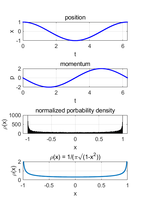
standard deviation momentum, sigmaP = 1.4142 **** WARNING the standard deviation sigmaP is wrong: ans should be sqrt(2) not 2 For the harmonic oscillator discussed in problems 1.11 and 1.12, we can
check the results using a numerical simulation where the position the
oscillator is computed at random times. QMG1J.m clear;
close all; clc % SETUP A = 1; %
amplitude k = 2; %
spring constant m = 2; %
mass w = sqrt(k/m); %
angular frequency T = 2*pi/w; %
period %
SIMULATION: randon times N = 1e5+1; %
Number of random times t = (T/1).*rand(1,N); x = A.*cos(w*t); v = -w.*A.*sin(w*t); p = m.*v; xmean =
mean(x); xstd =
std(x); pmean =
mean(p); pstd =
std(p); %
PROBABILITY and EXPECTATION VALUES xavg =
simpson1d(x,0,T)/T; x2avg = simpson1d(x.^2,0,T)/T; sigmaX = sqrt(x2avg - xavg^2); pavg =
simpson1d(p,0,T)/T; p2avg = simpson1d(p.^2,0,T)/T; sigmaP = sqrt(p2avg - pavg^2); rho = 1./(pi.*sqrt(A^2
- x.^2)); syms xs checkRHO =
int(1/(pi*sqrt(1-xs^2)),[-1 1]); % OUTPUT
disp('S simulation results
/ T probability & expectation results') fprintf('S number of random
times, N = %2.4e \n', N) fprintf('S average
position, <x> = %2.4f \n', xmean) fprintf('T average
position, <x> = %2.4f \n', xavg) fprintf('S standard
deviation position, sigmaX = %2.4f \n', xstd) fprintf('T standard
deviation position, sigmaX = %2.4f \n', sigmaX) fprintf('S average
momentum, <p> = %2.4f \n', pmean) fprintf('T average
momentum, <p> = %2.4f \n', pavg) fprintf('S standard
deviation momentum, sigmaP = %2.4f
\n', pstd) fprintf('T standard
deviation momentum, sigmaP = %2.4f
\n', sigmaP) fprintf('T CHECK rho
normalization = %2.4f \n', checkRHO) %
GRAPHICS figure(1) set(gcf,'units','normalized'); set(gcf,'position',[0.05 0.05 0.25 0.60]); set(gcf,'color','w'); FS = 14; subplot(4,1,1) xP = t; yP = x; plot(xP,yP,'b.','LineWidth',2) %xticks([L1:1:L2]) grid on xlabel('t') ylabel('x') title('position','FontWeight','normal') set(gca,'FontSize',FS) subplot(4,1,2) xP = t; yP = p; plot(xP,yP,'b.','LineWidth',2) %xticks([L1:1:L2]) grid on xlabel('t') ylabel('p') set(gca,'FontSize',FS) title('momentum','FontWeight','normal') subplot(4,1,3) R = linspace(-1,1,998); dR = R(2)-R(1); h = histogram(x,'BinEdges',R); c = get(h,'Values'); pD = c./(N*dR); check = simpson1d(pD,-1,1); ylim([0 1000]) grid on xlabel('x') ylabel('\rho(x)') set(gca,'FontSize',FS) title('normalized
porbability density','FontWeight','normal') fprintf('S Check normalization prob. density = %2.4f \n', check) subplot(4,1,4) plot(x,rho,'.') ylim([0 2]) grid on xlabel('x') ylabel('\rho(x)') title('\rho(x) =
1/(\pi\surd(1-x^2))','FontWeight','normal') set(gca,'FontSize',FS) >>
S
simulation results / T probability & expectation results S number
of random times, N = 1.0000e+05 S
average position, <x> = 0.0006
T
average position, <x> = 0.0003
S
standard deviation position, sigmaX = 0.7066 T
standard deviation position, sigmaX = 0.7067 S
average momentum, <p> = -0.0030
T
average momentum, <p> = -0.0045
S
standard deviation momentum, sigmaP
= 1.4153 T
standard deviation momentum, sigmaP
= 1.4151 T CHECK
rho normalization = 1.0000 S Check
normalization prob. density = 0.9772
|

|
QMG Problem 1.16 A particle is represented by the wave
function (a) Determine the
normalization constant A. (b) What is the
expectation value of x? (c) What is the
expectation value of p (d) Find the
uncertainty, (e) Find the
uncertainty. (f) Check that
your results are consistent with the uncertainty principle. |
|
QMG1K.m clear;
close all;clc % SETUP hbar =
1.05457182e-34; a = 1; x1 = -a; x2 = a; N = 9999; x = linspace(x1,x2,N); dx = x(2)-x(1); psi = (a^2 - x.^2); %
Normalize the wavefuntion AN = simpson1d(psi.^2,x1,x2); psi = psi./sqrt(AN); A = 1/sqrt(AN); check = simpson1d(psi.^2,x1,x2); % Most
likely postion to find the particle xM = x(psi == max(psi)); %
Expectation <x> fn = psi.*x.*psi; xavg =
simpson1d(fn,x1,x2); %
Expectation <x2> fn = psi.*x.^2.*psi; x2avg = simpson1d(fn,x1,x2); sigmaX = sqrt(x2avg - xavg^2); %
Momentum operator Gpsi =
gradient(psi,dx); fn = psi.*Gpsi; pavg = -1i*hbar*simpson1d(fn,x1,x2); G2psi = gradient(Gpsi,dx); fn = psi.*G2psi; p2avg = (-1i*hbar)^2*simpson1d(fn,x1,x2); sigmaP = sqrt(p2avg - conj(pavg).*pavg); % OUTPUT fprintf('Check
normalization: prob = %2.4f \n',
check) fprintf('Normalized
amplitude, A = %2.4f \n', A) fprintf('Most likely postion, xM = %2.4f \n', xM) fprintf('Expectation
value, <x> = %2.4f
\n', xavg) fprintf('Standard
deviation, sigmaX = %2.4f \n', sigmaX)
fprintf('Expectation value
<p> real = %2.4f imag =
%2.4f \n', real(pavg), imag(pavg)) fprintf('Standard
deviation, sigmaP/hbar =
%2.4f \n', sigmaP/hbar) fprintf('Uncertainty
Principle: sigmaX*sigmaP/hbar = %2.4f > 0.5 \n', sigmaX*sigmaP/hbar) %
GRAPHICS figure(1) set(gcf,'units','normalized'); set(gcf,'position',[0.35 0.05 0.25 0.35]); set(gcf,'color','w'); FS = 14; subplot(2,1,1) xP = x; yP = psi; plot(xP,yP,'b','LineWidth',2) grid on xlabel('x') ylabel('\psi') title('Wavefunctiopn','FontWeight','normal') set(gca,'FontSize',FS) subplot(2,1,2) xP = x; yP = psi.^2; plot(xP,yP,'b','LineWidth',2) grid on xlabel('x') ylabel('\psi^2') title('Probability
density','FontWeight','normal') set(gca,'FontSize',FS) >>
Check
normalization: prob = 1.0000 Normalized
amplitude, A = 0.9682 Most
likely postion, xM =
0.0000 Expectation
value, <x> = 0.0000 Standard
deviation, sigmaX = 0.3780 Expectation
value <p>
real = 0.0000
imag = 0.0000 Standard
deviation, sigmaP/hbar =
1.5811 Uncertainty
Principle: sigmaX*sigmaP/hbar = 0.5976 > 0.5 |

https://stemjock.com/griffithsqm3e.htm