|
MATLAB
RESOURCES INTRODUCTION
TO QUANTUM MECHANICS
3rd
Edition
David
J Griffiths & Darrel F Schroeter
Ian
Cooper matlabvisualphysics@gmail.com CHAPTER 2 THE SCHRODINGER EQUATION THE INFINITE SQUARE WELL DOWNLOAD DIRECTORY FOR MATLAB SCRIPTS simpson1d.m QMG2B.m Analytical
solution: Animated plot for the time evolution of the wavefunction and
probability density function. A plot of the wavefunction at the centre of the
potential well as a function of time. Calculations of the frequency and
period of the oscillation. The animation can be saved as a gif file. QMG2BB.m Numerical solution (finite difference
time development method): Animated plot for the time evolution of the
wavefunction and probability density function. A plot of the wavefunction at
the centre of the potential well as a function of time. Fourier transform of
the wavefunction at the centre of the potential well. Calculations of the
frequency and period of the oscillation. Calculation
of the total energy E Expectation value Frequency
Wavelength
& momentum Uncertainty
principal calculations Expectation values Standard deviations The animation
can be saved as a gif file. I will
only consider the Griffith Example 2.2, but in much more detail than is
required from the question. The techniques and methods used in my solution
will enable you to do most of the examples and problems in the section 2.2
The Infinite Square Well. Griffith
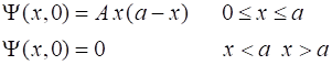
Example 2.2 A
particle in the infinite square well has the initial wave function for some
constant A. Find
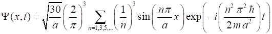
After
much tedious algebra, the solution for the wavefunction is However,
using the Matlab Script QMG2B.m, a greater insight to the solution can be
gained by an animation of the wavefunction and probability density function.
The width of the well is a = 1.0000
nm and the particle is an electron trapped inside the potential well. The
Script checks that the wavefunction is correctly normalized and computes the
period of the major peak in the wavefunction (n = 1).
Animation
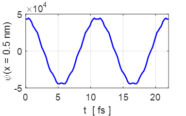
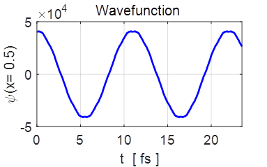
of the wavefunction and the probability density function.
The periodic motion of the wavefunction at the centre of the potential
well.
Notice the wobbles that occur in the functions, especially near the
extreme positions.
Left graph QMG2B.m (analytical solution)
Right graph QMG2BB.m (numerical solution) The
angular frequency
ang. frequency(n = 1) = 5.7129e+14 rad/s
period(n = 1) = 10.9982 fs
frequency(n = 1) = 9.0924e+13 Hz An
alternative way to solve this problem is by numerically solving the
Schrodinger equation using the finite difference time development method (FDTD) for the
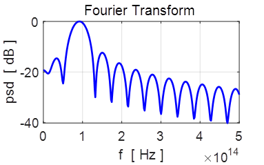
given initial value of the unnormalized wavefunction With the Script QMG2BB.m we can perform a Fourier transform on the
time variation of the wavefunction at the centre of the well to estimate the
frequency and period of the oscillation.
Fourier transform fpeak
= 9.23e+13 Hz period = 10.84 fs The period of oscillation calculated by
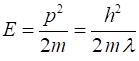
both methods are in good agreement with each other (PA = 11.0 fs PN = 10.8 fs). We can also estimate the total energy of the
system and since the potential energy is zero, the total energy equals the
kinetic energy of the electron. The wavelength is approximately equal to
twice the width of the well.
Wavelength
Electron mass me = 9.10938291x-31kg
Momentum
Total energy
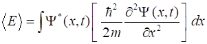
Kinetic energy T = E We can calculate the
total energy three ways: Wavelength
Frequency Expectation value Results
displayed in the Command Window: Fourier transform fpeak
= 9.23e+13 Hz period = 10.84 fs Total
energy E expectational value, <E> =
0.38 eV Fourier transform, Ef = h fpeak = 0.38 eV Theory, ET = p^2/2m = 0.38 eV Uncertainty
Principle dx = xSTD
= 1.89e-10 m dp = pSTD = 3.33e-25 m dx dp
= 6.30e-35 N.s hbar/2
= 5.27e-35 N.s.m dx dp
> hbar/2 The values of the total
energy computed in three different ways are all in agreement with each other. For the infinite square
well, the uncertainty principal is satisfied.
Animation of
wavefunction and probability density. QMG2BB.m. |