|
MATLAB
RESOURCES INTRODUCTION
TO QUANTUM MECHANICS
3rd
Edition
David
J Griffiths & Darrel F Schroeter
Ian
Cooper matlabvisualphysics@gmail.com CHAPTER 2 THE SCHRODINGER EQUATION THE HARMONIC OSCILLATOR DOWNLOAD DIRECTORY FOR MATLAB SCRIPTS simpson1d.m QMG23B.m HARMONIC OSCILLATOR:
TRUNCATED PARABOLIC POTENTIAL WELL In the
text by Griffiths, the treatment only discusses analytical methods on the
harmonic oscillator. In this approach, there is not much physics but lots of
mathematics. A better approach which gives more insight into the physics is
to use a numerical method which involves solving the time independent
Schrodinger equation for bound states using a matrix
method for finding the eigenvalues
and eigenvectors of the Hamiltonian operator. Nearly all the important
concepts of the harmonic oscillator can be investigated by this numerical
approach. The Matlab Scripts can be used as an alternative way of looking at
solutions to the examples and problems given in the Griffiths textbook. One of
the most important examples of applying the Schrodinger equation for a bound
particle is to consider the harmonic
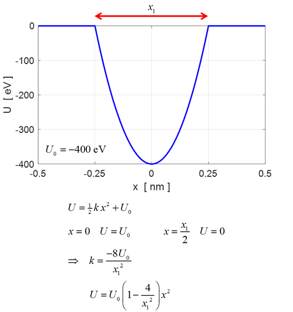
oscillator. The potential energy function
where k is the effective
spring constant, x is the
displacement from the equilibrium position and
Fig.
1. The potential energy
function used in the Script QMG23B.m to model the harmonic oscillator. The
Schrodinger equation that is solved by the matrix method is where
the Hamiltonian operator is expressed as a matrix In
solving this Schrodinger equation, all distances are measured in nanometres
and energies in electron-volts. Full details of the Matrix Method can be
viewed at https://d-arora.github.io/Doing-Physics-With-Matlab/mpDocs/qp_se_matrix.pdf For the
harmonic oscillator simulation, given the values for The
total energy spectrum for the harmonic oscillator with the potential shown in
figure 1 is given by
since
the total energy is measured from the bottom of the well and not from the
zero level. The ground sate energy is
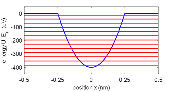
Figure 2
shows the total energy spectrum for the truncated parabolic potential well
for the harmonic oscillator. The
simulation predicts 13 bound states. The expectation values and the
theoretical values for the total energy of the system are shown in table 1.
This table is displayed in the Command Window of the Script QMG23B.m
Fig.
2. Potential energy
function and energy level spectrum for the harmonic oscillator. QMG23B.m Table
1. The expectation values
of the total energy predicted using the Matrix Method to find the eigenvalues
and eigenvectors and the theoretical values. No. bound
states found =
13 Quantum State / Eigenvalues En / Theory ET (eV) 1 -384.39
-384.38 2 -353.16
-353.15 3 -321.93
-321.92 4 -290.71
-290.69 5 -259.49
-259.46 6 -228.27
-228.23 7 -197.05
-197 8 -165.84
-165.77 9 -134.64
-134.54 10 -103.48
-103.31 11 -72.438
-72.078 12 -41.864
-40.847 13 -13.106
-9.6165 For the lower energy stationary states
there is excellent agreement between the eigenvalues and the theoretical
total energy values. But agreement gets worst at the higher the energy states
because the potential energy function is no longer parabolic in shape because
the potential energy used in the simulation is a truncated parabola. The
energy levels are equally spaced and the zero-point (ground) state is 15.6 eV
above the bottom of the potential well. The
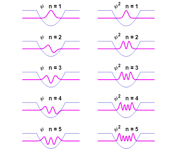
Matrix Method computes the eigenfunctions which are the stationary state
wavefunctions as shown in figure 2.
Fig. 2.
The wavefunctions and probability density functions for the first 5
stationary states for the harmonic oscillator. One can
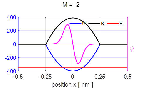
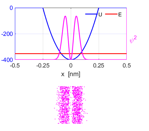
examine the properties of a single stationary state with the input variable M. Figure 3
shows the results for stationary state M = 2 for the potential energy U,
kinetic energy K, total
energy E, the
wavefunction
Fig. 3.
Stationary state M = 2. Each point in
the lower graph shows that position of the electron after each measurement
made on identical systems. Once the
wavefunction has been computed, it is a simple matter to calculate the
expectation values of:
and test
the uncertainty principle Table 2.
Expectation values and uncertainties for stationary state n
= 2. Quantum
number, n = 2 Energy, E
= -353.157 eV Total Probability
= 1 <x>
= -2.26336e-14 nm <x^2>
= 0.00365936 nm^2 <ip> = -1.43814e-40 N.s <ip^2>
= 6.83437e-48 N^2.s^2 <U>
= -376.58 eV <K>
= 23.4136 eV <E>
= -353.166 eV <K>
+ <U> = -353.166 eV deltax =
6.04926e-11 m
delta| = 2.61426e-24 N.s (dx dp)/hbar
= 1.4996
uncertainty principal satisfied Figure 5
illustrates the process of calculating the expectation value of the position
Fig.
5. Process of calculating
the expectation value of position The
Script also shows that two different stationary states are orthogonal to each
other Stationary
states M and N M = 1 N = 2 Integral = -0.0 Wavefunctions
are orthogonal The
quantum oscillator is strikingly different from its classical
counterpart—not only are the energies quantized, but the position
distributions have some bizarre features. For a classical particle,
oscillating in a parabolic shaped well, it travels very rapidly at the centre
of the well but slowly at its extreme positions. Therefore, the lowest
probability of locating the classical particle is at the centre of the well
and the highest probability is locating it at its extreme positions. However,
our electron in the ground state (M = 1), the maximum probability of locating
the bound electron is at the centre of the well and almost zero probability
at the extreme locations of the well (figure 6). Also, the probability of
finding the particle outside the classically allowed range (x greater
than the classical amplitude for the energy in question) is not zero.
Fig.
6. The bound electron does
not behave as a classical particle. The maximum probability of finding the
electron is at the centre of the well and not at the extreme positions (M = 1). However,
the electron’s behaviour is more like the classical particle at the
highest quantum numbers for the bound electron (figure 7). Figure 8 shows the
probability density for a classical particle.
Fig.
7. Probability density
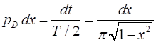
function We can calculate the probabilty density function for a
classical particle oscillating with simple harmonic motion between xC =-1 and xC =
+1. If the oscillator spends an infinitesimal
amount of time dt in the
vicinity dx of a
given x value, then
the probability
Fig.
8. Probability density function
for a classical particle executing simple harmonic motion. We can
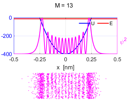
animate the time evolution of the wavefunctions. Figure 9 shows the
wavefunction and the probability distribution for the stationary state M =
13. For the stationary state, the probability distribution is time
independent.
Fig.
9. Wavefunction and probability
distribution for the stationary state qn = 13. Linear
combination of stationary states We can consider
a compound state which is a superposition of two stationary states with
quantum numbers M and N. The normalized wavefunction can be expressed as
This
compound wavefunction is not time independent as shown in the animation
(figure 10) for M = 1 and N = 2. The probability density sloshes back and
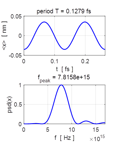
forth with simple harmonic motion. Thus, the expectation value also varies
sinusoidally as shown in figure 12.
Fig. 11.
The wavefunction with M = 1 and N = 2 and its probability distribution are time
dependent.
Fig 12.
The sinusoidal variation in the expectation value for position and its
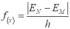
Fourier transform. The
theoretical values for the oscillation of the expectation value of x and its
period are
The
values from the numerical computation and Fourier transform are The
theoretical values and the simulations values are in reasonable agreement
with each other. If If |