|
MATLAB
RESOURCES QUANTUM
MECHANICS
Ian
Cooper matlabvisualphysics@gmail.com TIME DEPENDENT SCHRODINGER EQUATION FINITE DIFFERENCE TIME DEVELOPMENT METHOD DOWNLOAD DIRECTORY FOR MATLAB SCRIPTS The Schrodinger Equation is the basis of
quantum mechanics. The state of a particle is described by its wavefunction We will consider solving the [1D]
time dependent Schrodinger Equation
using the Finite
Difference Time Development Method (FDTD). The one-dimensional time
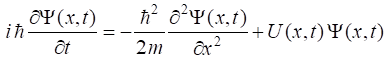
dependent Schrodinger equation for a particle of mass m
is given by (1) where The wavefunction is
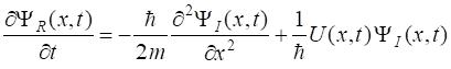
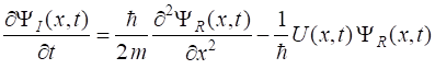
best expressed in terms of its real and imaginary parts (2) Inserting equation 2
into equation 1 and separating real and imaginary parts results in the
following pair of coupled equations (3a) (3b) We can now
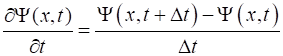
apply the finite difference approximations for the first derivative in time
and the second derivative in space. The time step is Time
Grid
positions Wavefunction
is calculated at each time step nt
where the
symbol y is used for the wavefunction in the coding
of the Script. (4) (5) The second
derivative of the wavefunction given by equation 5 is not defined at the
boundaries. The simplest approach to solve this problem is to set the
wavefunction at the boundaries to be zero. This can cause problems because of
reflections at both boundaries. Usually, a simulation is terminated before
the reflections dominate. Substituting
equations 4 and 5 into equations 3a and 3b and applying the discrete times
and spatial grid gives the latest value of the wavefunction expressed in
terms of earlier values of the wavefunction at each time step are calculated
from equations 6a and 6b (6a) (6b)
where the
constants C1 and C2
are (7) for nt = 1 : Nt-1 for nx = 2 : Nx
- 1 yR(nx) = yR(nx) - C1*(yI(nx+1)-2*yI(nx)+yI(nx-1))
+ C2*U(nx)*yI(nx); end psiR(nt+1,:) = yR; for nx = 2 : Nx-1 yI(nx) = yI(nx) + C1*(yR(nx+1)-2*yR(nx)+yR(nx-1))
- C2*U(nx)*yR(nx); end psiI(nt+1,:) = yI; end for nt = 2:Nt psiI(nt,:) = 0.5*(psiI(nt,:) + psiI(nt-1,:)); end The potential U is given in electron-volts (eV) and to
convert to joules, the charge of the electron e
is included in
the equation for the constant C2. In equations 6a and 6b, the y variables on the RHS
gives the values of the wavefunction at time (8) It is a
relatively easy task to model an electron in a system with a potential energy
function |