|
MATLAB
RESOURCES QUANTUM
MECHANICS
Ian
Cooper matlabvisualphysics@gmail.com WAVEFUNCTION: OBSERVABLES, EXPECTATION VALUES, UNCERTAINTIES, HEISENBERG UNCERTAINTY PRINCIPLE DOWNLOAD DIRECTORY FOR MATLAB SCRIPTS simpson1d.m used to
evaluate all [1D] integrals QMG24D.m Propagation
of a quantum-mechanical Gaussian pulse (example
of calculating expectation values) EXPECTATION VALUES
OF OBSERVABLES The wavefunction The expectation
value of an observable quantity A is the
quantum-mechanical prediction for the mean value of A. We will consider a particle
to be an electron and that we know the wavefunction (1) The
quantity The
probability of finding the electron in the region from (2) Consider
N identical systems, each containing an
electron. We make N identical measurements on each system
of the physical parameter A. In a
quantum system, each measurement is different. From our N measurements, we can calculate the mean value The
mean value of an observable quantity A is
found by calculating its expectation
value (3) where
and
its uncertainty is the standard deviation of A. The uncertainty (4) (5) The
quantity For
our [1D] system, a particle in any state must have an uncertainty in position
(6) The
Heisenberg Uncertainty Principle tells us that it is impossible to find a
state in which a particle can has definite values in both position and
momentum. Hence, the classical view of a particle following a well-defined
trajectory is demolished by the ideas of quantum mechanics. Table 1
gives a summary of the most important operators for [1D] quantum systems.
Expectation values maybe time dependent. |


Table 1. Observables, Operators
and Expectation values
|
Observable |
Operator |
Expectation Value |
|
probability |
1 |
|
|
position |
x |
|
|
x2 |
x2 |
|
|
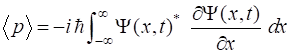
momentum |
|
|
|
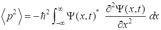
p2 |
|
|
|
Potential
energy |
U |
|
|
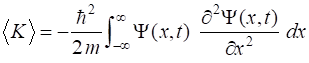
Kinetic
energy |
K |
|