A NUMERICAL APPROACH TO THE PHYSICS OF THE
ENVIRONMENT AND CLIMATE
Ian Cooper
matlabvisualphysics@gmail.com
CHAOS IN THE ATMOSPHERE
MATLAB
Download directory
https://drive.google.com/drive/u/3/folders/1j09aAhfrVYpiMavajrgSvUMc89ksF9Jb
https://github.com/D-Arora/Doing-Physics-With-Matlab/tree/master/mpScripts
SCRIPTS
atmDDP.m
Uses ode45 to solve the equation of motion for
a damped driven pendulum (DDP). The main input
variable is the drive strength ![]() . The graphical
output plots are: drive stimulus vs
time; angular displacement vs time; angular frequency vs time; phase space;
Fourier transform of the angular displacement. You need to download the Script simpson1d.m to calculate
the Fourier transform by the direct integration of the Fourier integral.
. The graphical
output plots are: drive stimulus vs
time; angular displacement vs time; angular frequency vs time; phase space;
Fourier transform of the angular displacement. You need to download the Script simpson1d.m to calculate
the Fourier transform by the direct integration of the Fourier integral.
The nonlinear ODE for the DDP
system is extremely sensitive to the model’s parameters and initial
conditions. All input parameters much be chosen with care. Values mostly used
in the simulations are those used by J.R. Taylor
in his excellent book Classical Physics.
Time
space: from ~ 10 s to ~ 10 000 s
Drive
strength ![]() : ~ 0.2 to ~ 2.0
: ~ 0.2 to ~ 2.0
Drive
period TD (cycle
time): TD = 1.00
s ![]()
Natural
frequency: ![]()
Damping
parameter: ![]() or
or ![]()
Initial condition
for angular displacement: ![]() or
or ![]() rad
rad
Initial condition
for angular frequency:
![]() rad.s-1
rad.s-1
ode45 options: opts = odeset('RelTol',1e-10);
atmPendulumPS.m
A Poincare
section for a given drive
strength ![]() is plotted by
solving the ODE with ode45 function. To construct the Poincare section for
chaotic motion, many thousands of time steps have to be used.
is plotted by
solving the ODE with ode45 function. To construct the Poincare section for
chaotic motion, many thousands of time steps have to be used.
atmPendulumBD.m
A bifurcation
diagram is constructed by solving
the equation of motion for a range of drive strengths ![]() . After the transient oscillation have decayed, peak values
in the angular displacement are used to plot the bifurcation diagram. This
method is only suitable for a limited range of
. After the transient oscillation have decayed, peak values
in the angular displacement are used to plot the bifurcation diagram. This
method is only suitable for a limited range of ![]() which is less than some critical value.
which is less than some critical value.
atmPendulumBDS.m
A bifurcation
diagram is constructed by solving
the equation of motion for a range of drive strengths ![]() . For each
. For each ![]() , the angular displacements in successive drive cycles are
plotted.
, the angular displacements in successive drive cycles are
plotted.
atmPendulum2A.m
Lyapunov
Exponent of a dynamical system is a quantity that
characterizes the rate of separation of infinitesimally close trajectories.
INTRODUCTION
It is without question that accurate weather
predictions are of the utmost importance. To forecast the weather, it is
necessary to use complex numerical models. In the 1960s Edward Lorenz while
developing his models on weather prediction, made a startling discovery leading
to the discovery of chaos. Even though a system may be completely
deterministic, chaotic systems are extremely sensitive the initial conditions.
Although we will not model chaotic weather
systems, we can gain much insight to chaotic systems by studying the behaviour
of a very simple system, the damped driven
pendulum (DDP).
For a system to exhibit chaos its equations
of motion must be nonlinear.
However, nonlinearity does not guarantee chaos. To illustrate many
of the principles of chaotic motion, we will consider the nonlinear system of a
damped driven pendulum as described by Taylor in his book Classical Mechanics.
The equation of motion for the pendulum is
(1) 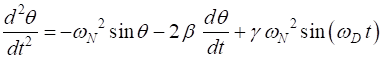
where
![]() angular
displacement [rad]
angular
displacement [rad]
t
time [s]
![]() angular frequency
[rad.s-1]
angular frequency
[rad.s-1]
![]() damping
coefficient [s-1]
damping
coefficient [s-1]
![]() driving
strength [rad-1]
driving
strength [rad-1]
![]() angular
frequency of the driving signal [rad.s-1]
angular
frequency of the driving signal [rad.s-1]
g
acceleration due to gravity
[g = 9.80 m.s-2]
L length of
pendulum [m]
The angular frequency ![]() is the time rate of change of the
angular displacement
is the time rate of change of the
angular displacement ![]() and T is the period and the f of oscillation
and T is the period and the f of oscillation
(2) 
The natural angular frequency ![]() and
period
and
period ![]() of the
system for a simple pendulum are
of the
system for a simple pendulum are
(3) 
The ODE equation 1 is solved using the
Matlab function ode45 with the default parameters (S.I.
units)
![]()
![]()
![]()
For some values of the parameters, equation
1 does lead to chaotic motion. Note, the superposition principle does not apply
to nonlinear systems.
1 Free
motion of the pendulum with a small initial displacement
atmDDP.m
![]()
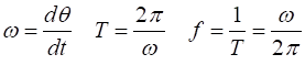
The results of the simulation are shown in figures 1.1 and 1.2.
Fig. 1.1 Simple harmonic motion for small
amplitude free motion of the pendulum.
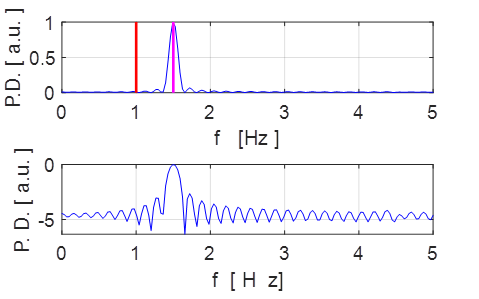
Fig. 1.2 Power density plot: Fourier
transform of the angular displacement.
fN
= 1.50 Hz magenta
fD
= 1.00 Hz red
The pendulum oscillates at its natural
frequency (1.5 Hz) and its motion is described as simple harmonic motion (SHM). Figure 2 displays the Fourier Transform (calculated by direction integration of the
Fourier Transform integral). For
small amplitude oscillation the pendulum corresponds to a linear system.
2 Free motion of the
pendulum with a large initial displacement
atmDDP.m
![]()
The results are shown in figures 2.1 and
2.2. The motion is no longer SHM. The motion is
periodic with frequency 0.68 Hz and period 1.47 s. The oscillation frequency is
lower and its period longer compared with the small amplitude SHM. The peaks
in the angular displacement plot are flatter than for SHM
as the restoring force is less than for SHM ![]() .
.
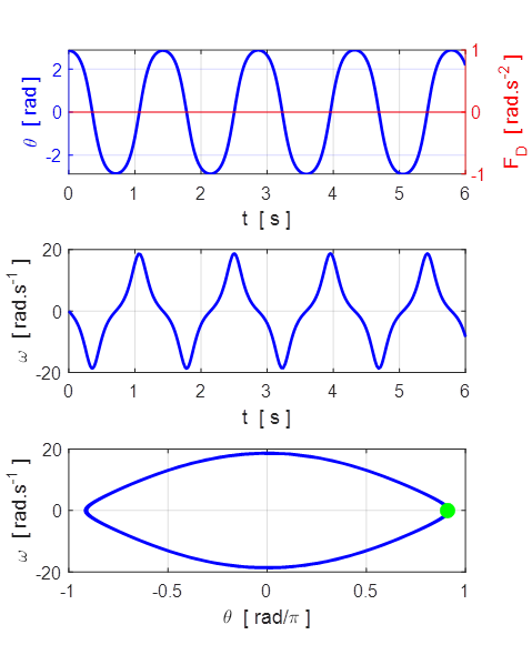
Fig. 2.1 Large amplitude free motion of the
pendulum. The motion is periodic but not simple harmonic motion.
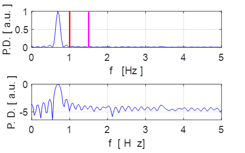
Fig. 2.2 Fourier Transform spectrum: peak oscillation frequency f = 0.68 Hz.
fN
= 1.50 Hz magenta
fD
= 1.00 Hz red
3 Free
motion of the pendulum and small damping
atmDDP.m
Small initial
angular displacement
![]()
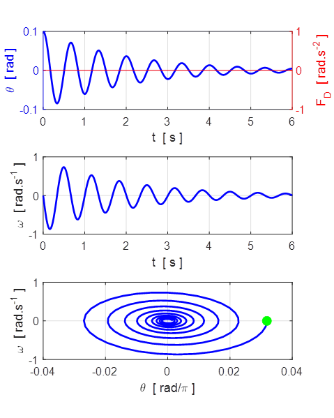
Fig. 3.1 Small amplitude damped
oscillations.
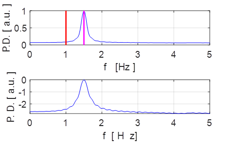
Fig. 3.2 Fourier Transform spectrum: peak oscillation frequency f = 1.00 Hz.
fN
= 1.50 Hz magenta
fD
= 1.00 Hz
Large initial
angular displacement
![]()
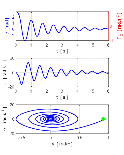
Fig. 3.3 Large amplitude damped
oscillations.
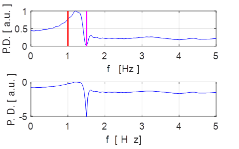
Fig.3.4 Fourier Transform spectrum: peak oscillation frequency f = 1.20 Hz.
fN
= 1.50 Hz magenta fD = 1.00 Hz
When the system is damped, the frequency
band width is wider than the for the undamped system.
The [2D] plot of ![]() is
called the phase space or state space
plot as the two variables
is
called the phase space or state space
plot as the two variables ![]() and
and ![]() completely defines the state of the
pendulum. A phase space orbit is simply the trajectory of the two variables
completely defines the state of the
pendulum. A phase space orbit is simply the trajectory of the two variables ![]() and
and ![]() as time
evolves. A closed orbit which
is an elliptical attractor always evolves in a clockwise sense as shown in
the above phase space plots (the green dot shows
the initial conditions). The time to complete one closed orbit is the period of
the oscillation.
as time
evolves. A closed orbit which
is an elliptical attractor always evolves in a clockwise sense as shown in
the above phase space plots (the green dot shows
the initial conditions). The time to complete one closed orbit is the period of
the oscillation.
4 Damped
Driven Pendulum ( DDP )
atmDDP.m
The DDP system is
excited by some external sinusoidal driving stimulus as shown in figure 4.1.
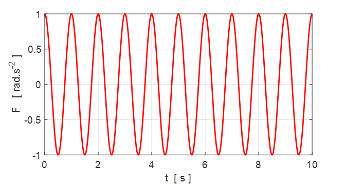
Fig. 4.1 A sinusoidal stimulus drives the
oscillations of the DDP system with frequency fD = 1.00 Hz and period TD
= 1.00 s (the drive cycle).
The response of the DDP
system can be studied by changing the input model parameters. Plots can be made
for the time evolution of the system, phase space, Poincare sections and
bifurcation diagrams.
PERIODIC OSCILLATIONS
The default parameters mainly are used for
each simulation. Only the driving force strength ![]() is successively
increased.
is successively
increased.
Relatively weak driving
strength ![]()
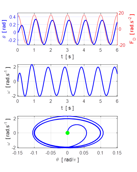
Fig. 4.2 The motion of the DDP for relatively weak driving strength ![]() .
After the initial transient lasting about 3 cycles (3 s), the motion is SHM with a period equal to the driving period,
.
After the initial transient lasting about 3 cycles (3 s), the motion is SHM with a period equal to the driving period, ![]() .
After the initial transient motion, the orbit in the phase space is an ellipse
(the attractor).
.
After the initial transient motion, the orbit in the phase space is an ellipse
(the attractor).
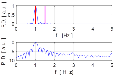
Fig. 4.3 Weak driving strength ![]() . Fourier Transform spectrum: peak oscillation frequency f = 1.00 Hz.
. Fourier Transform spectrum: peak oscillation frequency f = 1.00 Hz.
fN
= 1.50 Hz magenta fD =
1.00 Hz red
We see that the driver and the response have
the same period. Something which intuition from linear problems would say is
obvious. The
response has two regimes: (1) the decay of an initial transient motion and (2)
the steady oscillations at the frequency of the driving signal. The amplitude
of the response depends upon the energy balance between the energy supplied by
the external driving force and the energy dissipated by the system due to the
damping. The phase space plot exhibits a regular orbit which is independent of
the initial conditions except for the initial transients which does depend upon
the initial conditions. The motion approaches a unique attractor in which the pendulum
oscillates sinusoidally with exactly the same frequency as the driving force.
In
conclusion for the motion of the linear DDP with a
sinusoidal driving force:
(1) There is
a unique attractor which the motion approaches, irrespective of the initial
conditions applied.
(2) The
motion of the attractor is itself sinusoidal with frequency exactly matching
the drive frequency.
We can now increase the driver strength to
so the approximation ![]() is no longer valid.
is no longer valid.
Weak driving input ![]()
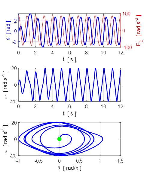
Fig. 4.4 Motion of DDP
for ![]() . After 4 cycles (4 s) the motion settles down
to a regular oscillation that looks like sinusoidal with a period equal to the
driving frequency. However, the regular oscillations are not sinusoidal but the
curve is flatter at the extremes.
. After 4 cycles (4 s) the motion settles down
to a regular oscillation that looks like sinusoidal with a period equal to the
driving frequency. However, the regular oscillations are not sinusoidal but the
curve is flatter at the extremes.
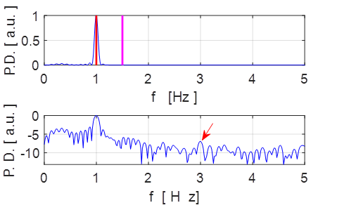
Fig. 4.5 DDP
spectrum for ![]() . Most of the energy supplied by the driving
force to the DDP system excites the fundamental
frequency (driving frequency fD = 1.00 Hz). A small amount of energy also
excites the 3rd harmonic at a frequency of 3.00 Hz.
. Most of the energy supplied by the driving
force to the DDP system excites the fundamental
frequency (driving frequency fD = 1.00 Hz). A small amount of energy also
excites the 3rd harmonic at a frequency of 3.00 Hz.
The boundary between weak and strong driving
stimulus is around ![]() .
.
When we increase the driving strength by a
small amount, we find more harmonics excited.
Strong driving
strength ![]()
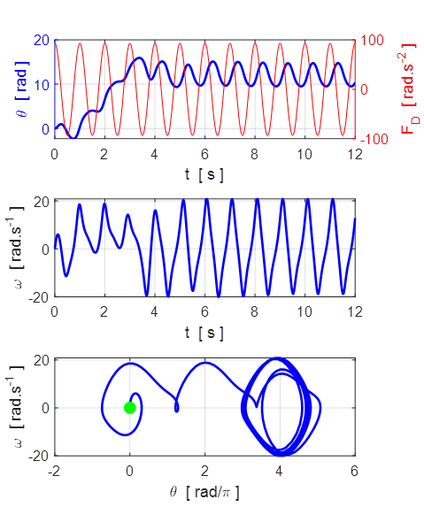
Fig. 4.6 Motion of DDP
for ![]() . After 4 cycles (4 s) the motion settles down
to a regular oscillation with a period equal to the driving frequency that has
a DC component.
. After 4 cycles (4 s) the motion settles down
to a regular oscillation with a period equal to the driving frequency that has
a DC component.
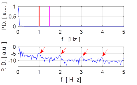
Fig. 4.7 As the driving strength increases
more energy goes into the harmonics. After one cycle of the driving signal, all
the harmonics will also have undergone multiple complete cycles. Hence, the
motion made up of all the harmonics will still oscillate at the driving
frequency.
The motion for strong stimuli is very
different from the weak stimuli. In the first 5 s of the motion, the pendulum
swings through about and two and half counter clockwise rotations. Then in the
next 2 s it swings from ![]() to
to
![]() then settles down to oscillate almost
sinusoidally around
then settles down to oscillate almost
sinusoidally around ![]() which is really
which is really ![]() . This means that the pendulum has made one
complete revolution since t = 0
before oscillating backwards and forwards about
. This means that the pendulum has made one
complete revolution since t = 0
before oscillating backwards and forwards about ![]() .
.
From the graphs we cannot be completely sure
that the motion is exactly periodic. One way to test this is to examine the
peaks in the angular displacement plot more carefully. This is easily done
using the Matlab function findpeaks. The results are displayed as a table
in the Command Window for the times of the peaks and their magnitudes.
% Find peaks for
calc of period if flagP = 1
flagP = 1;
if flagP == 1
[pks, loc] = findpeaks(X,t);
TP = (loc(end) - loc(end-2))/2;
end
for c = 1 : length(pks)
fprintf(' %2.3f %2.3f \n', loc(c),
pks(c))
end

From the table of results, it is clear that
after the initial transient oscillations have decayed, the oscillation period
is 1.0 s and a constant peak height of ~14.75. So, there is strong evidence
(not a proof) that a periodic attractor is approach with a period exactly equal
to the driving force.
5 PERIOD DOUBLING
atmDDP.m
The most noticeable feature for a larger
value of the drive strength ![]() is that the trajectory is very different
if you use different initial conditions. After the initial irregular transient
oscillations in angular displacement, they appear to be at least approximately
sinusoidal with a period equal to the drive period. However, on close
examination you will notice that alternate peaks (or troughs) are not all of
the same height.
is that the trajectory is very different
if you use different initial conditions. After the initial irregular transient
oscillations in angular displacement, they appear to be at least approximately
sinusoidal with a period equal to the drive period. However, on close
examination you will notice that alternate peaks (or troughs) are not all of
the same height.
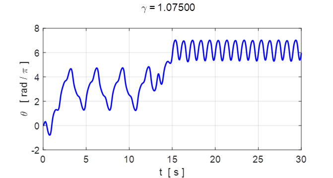
Fig. 5.1 Angular displacement ![]() .
.
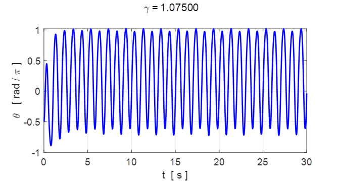
Fig. 5.2 Angular displacement ![]() .
.
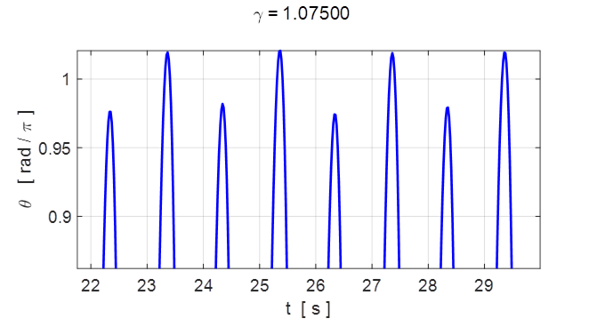
Fig. 5.3 Expanded view of angular
displacement ![]() in figure 5.2.
The attractor is approximately sinusoidal with alternate peaks having different
heights, repeating themselves every two drive cycles (2 s).
in figure 5.2.
The attractor is approximately sinusoidal with alternate peaks having different
heights, repeating themselves every two drive cycles (2 s).
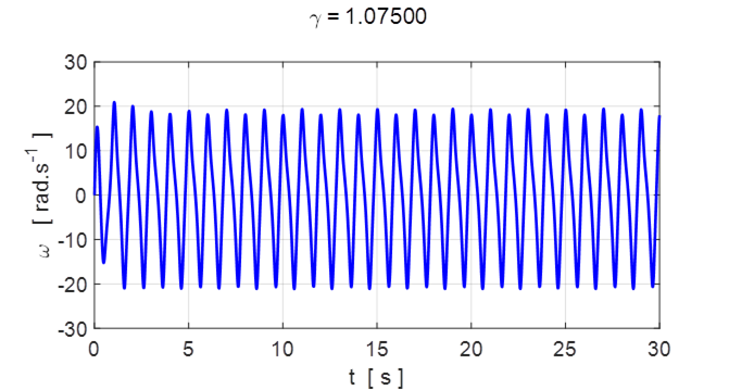
Fig. 5.4 Angular velocity ![]() . Note:
double peaks. After the initial fluctuations, the
oscillations settle down to an attractor that is approximately sinusoidal.
. Note:
double peaks. After the initial fluctuations, the
oscillations settle down to an attractor that is approximately sinusoidal.
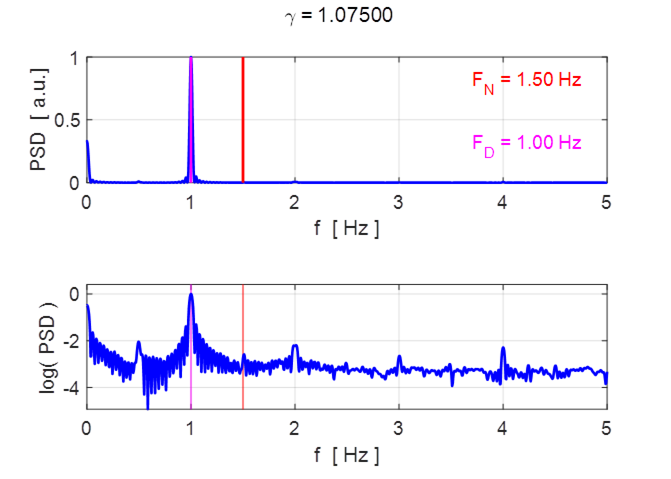
Fig. 5.6 Frequency spectrum of angular
displacement ![]() .
.
Table 1 Time between adjacent peaks of
different height is 1.0 s and the pattern repeats itself every 2.0 s.
![]()
You can see from the enlargement shown in
figure 3 and Table 1, the peaks alternate between two distinct heights and this
pattern persists. This pattern no longer repeats itself at the period of the
driver, but rather the period of the motion is equal to twice the period of the
driver. This is referred to as period doubling. Therefore, there is a
subharmonic of the drive frequency ![]() . The
Fourier transform shown in figure 5.6 shows a dominant peak at the drive
frequency (1.0 Hz) and small peaks at the subharmonic (0.5 Hz) and the 2nd
harmonics 2 (2.0 Hz), 3rd harmonic (3.0 Hz), and 4th harmonic
(4.0 Hz).
. The
Fourier transform shown in figure 5.6 shows a dominant peak at the drive
frequency (1.0 Hz) and small peaks at the subharmonic (0.5 Hz) and the 2nd
harmonics 2 (2.0 Hz), 3rd harmonic (3.0 Hz), and 4th harmonic
(4.0 Hz).
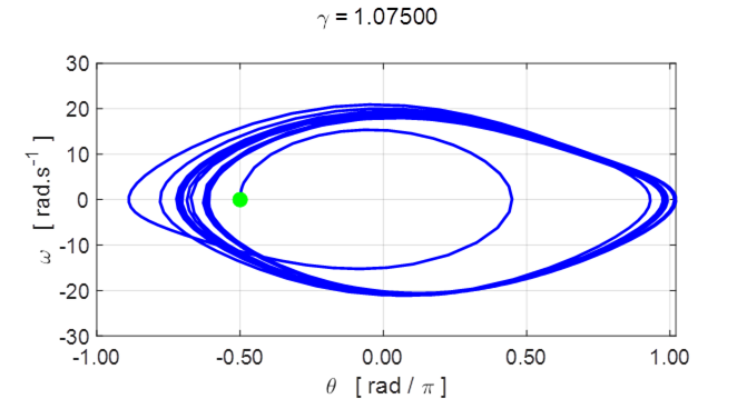
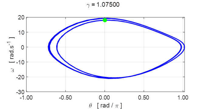
Fig. 5.7 Phase space orbits. ![]() It shows the
periodic attractor with period 2 (2 s). The bottom graph shows the two distinct
loops each lasting one drive cycle (1 s) in the orbit for the time from 40 s to
50 s when the transient oscillations have fully decay.
It shows the
periodic attractor with period 2 (2 s). The bottom graph shows the two distinct
loops each lasting one drive cycle (1 s) in the orbit for the time from 40 s to
50 s when the transient oscillations have fully decay.
When the transient oscillations have fully
decayed, a closed orbit evolves in the phase space plot that has two distinct
orbits can be seen, so the motion repeats itself every two cycles, that is, it
has period 2.
6 Transition to non-sinusoidal
motion
atmPendulumMF.m
![]()
In Example 5, even though there was a
doubling of the period due to the alternating peaks, the dominant motion was
still approximately sinusoidal at the frequency of the driving force. When the
driving strength is slightly increased, a subharmonic term dominates and the
motion is no longer sinusoidal. The motion settles down to the periodic
attractor which has a period of three times the driver period (3 s).
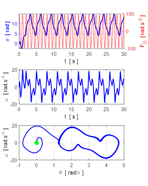
Fig. 6.1 DDP ![]() . After the initial transience, the motion
settles down to a periodic attractor with a period of three times the drive
period (3 s).
. After the initial transience, the motion
settles down to a periodic attractor with a period of three times the drive
period (3 s).
![]()
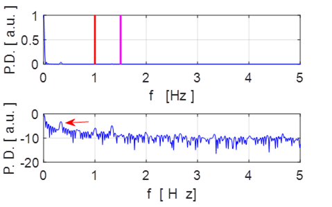
Fig. 6.2. Strong driver strength ![]() . The subharmonic 1/3 is excited. The motion
is non-sinusoidal but periodic with a period three times the drive period. he
1/3 Hz subharmonic dominates.
. The subharmonic 1/3 is excited. The motion
is non-sinusoidal but periodic with a period three times the drive period. he
1/3 Hz subharmonic dominates.
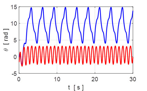
Fig. 6.3. Two solution for the DDP
with different initial conditions ![]() but with the same
drive strength. The motions are entirely different.
but with the same
drive strength. The motions are entirely different.
For the case of linear DDP,
the attractor is independent of the initial conditions. This is not the case
for nonlinear DDP. For a nonlinear oscillator,
different initial conditions can lead to very different trajectories. For the
motion with the initial condition ![]() the
period of oscillation is 3 s. When the initial condition was
the
period of oscillation is 3 s. When the initial condition was ![]() the period is actually 2 s with the peaks
and troughs having slightly different heights.
the period is actually 2 s with the peaks
and troughs having slightly different heights.
7 Period doubling cascade
atmPendulumMF.m
Figure (7.1) shows a sequence of four plots
for the DDP with increasing drive strength ![]() for the same
initial conditions
for the same
initial conditions ![]() .
.
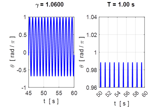
![]() Motion settles down to steady
oscillations at the same frequency of the drive excitation. The attractor has a
period of 1.00 s. The expanded view shows that all the peaks have the same
height.
Motion settles down to steady
oscillations at the same frequency of the drive excitation. The attractor has a
period of 1.00 s. The expanded view shows that all the peaks have the same
height.
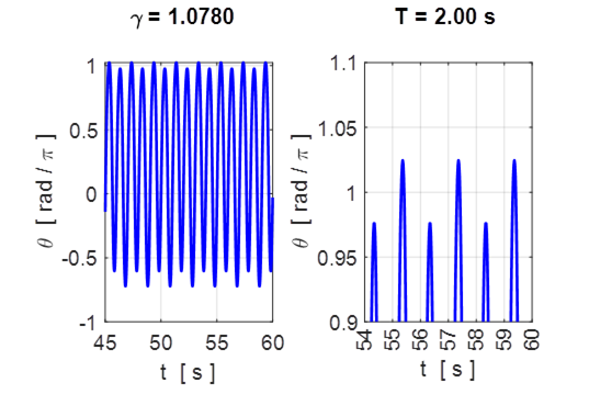
![]() Motion settles down to steady
oscillations at the same frequency of the drive excitation. But now, the peaks
are not all the same height. The maxima alternate between two fixed heights, so
the attractor has a period of 2.0 s.
Motion settles down to steady
oscillations at the same frequency of the drive excitation. But now, the peaks
are not all the same height. The maxima alternate between two fixed heights, so
the attractor has a period of 2.0 s.
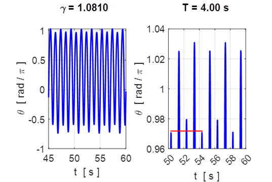
![]() Motion settles down to steady
oscillations at the same frequency of the drive excitation. But now, the peaks
are not all the same height. The maxima alternate between four fixed heights,
so the attractor has a period of 4.0 s.
Motion settles down to steady
oscillations at the same frequency of the drive excitation. But now, the peaks
are not all the same height. The maxima alternate between four fixed heights,
so the attractor has a period of 4.0 s.
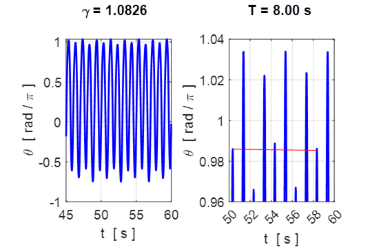
![]() Motion settles down to steady
oscillations at the same frequency of the drive excitation. But now, the peaks
are not all the same height. The maxima alternate between eight fixed heights,
so the attractor has a period of 8.0 s. the pattern repeats itself every 8
drive cycles.
Motion settles down to steady
oscillations at the same frequency of the drive excitation. But now, the peaks
are not all the same height. The maxima alternate between eight fixed heights,
so the attractor has a period of 8.0 s. the pattern repeats itself every 8
drive cycles.
Fig. 7.1 A period doubling cascade due to
increasing drive strength ![]() .
.
These four pictures show a period-doubling cascade. Increasing the
drive strength would produce further doublings of the period 16, 32, … , ![]() . It can be difficult to find the threshold
drive frequencies between doublings. The doublings that occur get faster and
faster as the drive strength
. It can be difficult to find the threshold
drive frequencies between doublings. The doublings that occur get faster and
faster as the drive strength ![]() is increased. This period-doubling in
many nonlinear systems has been observed, for example, electrical circuits,
chemical reactions, and balls bouncing on oscillating surfaces.
is increased. This period-doubling in
many nonlinear systems has been observed, for example, electrical circuits,
chemical reactions, and balls bouncing on oscillating surfaces.
8 CHAOS and sensitivity to
initial conditions
atmPendulumMF.m
For drive strengths greater than about a
critical value of ![]() ,
the solution is now not even periodic at all! In linear theory, a damped system
driven periodically must eventually respond periodically at the driving
frequency and the oscillations independent upon the initial conditions. In this case for drive strengths greater
than the critical value, the DDP nonlinear system
will oscillate forever without ever repeating – it is chaotic.
,
the solution is now not even periodic at all! In linear theory, a damped system
driven periodically must eventually respond periodically at the driving
frequency and the oscillations independent upon the initial conditions. In this case for drive strengths greater
than the critical value, the DDP nonlinear system
will oscillate forever without ever repeating – it is chaotic.
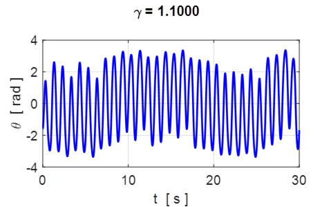
Fig. 8.1 Chaos. Initial conditions ![]()
The case for ![]() with initial conditions
with initial conditions ![]() , is shown in figure 8.1. The DDP
is obviously trying to oscillate at the drive frequency fD
= 1.00 Hz. Nevertheless, the actual oscillations wander around erratically
without ever repeating themselves. This erratic
and non-periodic motion is one of the chief features of chaotic
motion.
, is shown in figure 8.1. The DDP
is obviously trying to oscillate at the drive frequency fD
= 1.00 Hz. Nevertheless, the actual oscillations wander around erratically
without ever repeating themselves. This erratic
and non-periodic motion is one of the chief features of chaotic
motion.
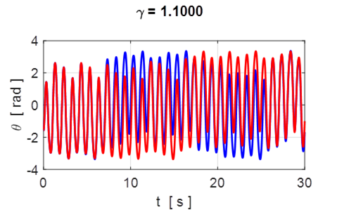
Fig. 8.2 Chaos. Initial conditions
![]()
![]()
The other defining feature of chaos is that
a trajectory is extremely sensitive
to the initial conditions as shown in
figure 8.2 where the initial displacement is decreased by only 0.5%. For the
duration of about 7 drive cycles, the motions are almost identical, then they
follow different trajectories. This makes it an impossibility to predict the
trajectories for chaotic motion.
9 Lyapunov Exponents
atmPendulum2A.m
Figures 9.1 shows two motions of the
pendulum with a small driving force ![]() with
different initial conditions
with
different initial conditions ![]() . The upper graph shows the angular
displacements as functions of time and the lower graph, the difference in the
angular displacements
. The upper graph shows the angular
displacements as functions of time and the lower graph, the difference in the
angular displacements ![]() .
.
![]() is
plotted on a logarithmic scale.
is
plotted on a logarithmic scale.
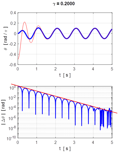
Fig. 9.1 Logarithmic plot of ![]() ,
the separation of two identical DDPs with a weak
driving force
,
the separation of two identical DDPs with a weak
driving force ![]() that were released with different initial
angular displacements
that were released with different initial
angular displacements ![]() .
.
It is clear from figure 9.1 the maxima in
the log scale for ![]() decrease linearly, hence
decrease linearly, hence ![]() decays
exponentially, dropping 5 orders of magnitude in the first five drive cycles.
In the linear regime, the separation
decays
exponentially, dropping 5 orders of magnitude in the first five drive cycles.
In the linear regime, the separation ![]() of two
identical DDPs with different initial conditions,
decreases exponentially with time. Linear oscillators are insensitive to the
initial conditions. So, to make accurate predictions, you only need to know the
initial conditions to the same accuracy.
of two
identical DDPs with different initial conditions,
decreases exponentially with time. Linear oscillators are insensitive to the
initial conditions. So, to make accurate predictions, you only need to know the
initial conditions to the same accuracy.
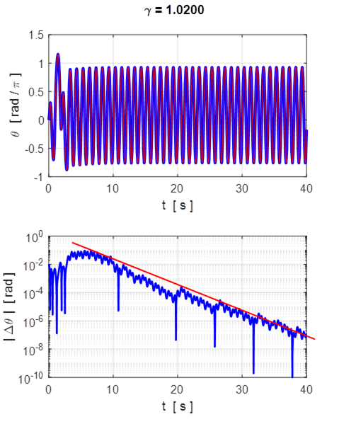
Fig. 9.2 Logarithmic plot of ![]() ,
the separation of two identical DDPs with a moderate
driving force
,
the separation of two identical DDPs with a moderate
driving force ![]() that were released with different initial
angular displacements
that were released with different initial
angular displacements ![]() .
.
With a moderate drive strength ![]() the
motions are periodic and their trajectories converge with
the
motions are periodic and their trajectories converge with ![]() decaying exponentially. For the
motion governed by a moderate driving signal, the sharp dips in the
decaying exponentially. For the
motion governed by a moderate driving signal, the sharp dips in the ![]() plot occur when one of the pendulums
reaches a turning point, following which
plot occur when one of the pendulums
reaches a turning point, following which ![]() will vanish since the two pendulums will
cross each other. You will notice that
will vanish since the two pendulums will
cross each other. You will notice that ![]() decreases
steady with time such that
decreases
steady with time such that ![]() (ignoring
the dips).
This means that the motion of the pendulum is predictable. Knowledge of the
motion of the first pendulum enables you to predict the motion of the second
pendulum even though you don’t know the second pendulum’s initial
conditions when the forcing is small to moderate.
(ignoring
the dips).
This means that the motion of the pendulum is predictable. Knowledge of the
motion of the first pendulum enables you to predict the motion of the second
pendulum even though you don’t know the second pendulum’s initial
conditions when the forcing is small to moderate.
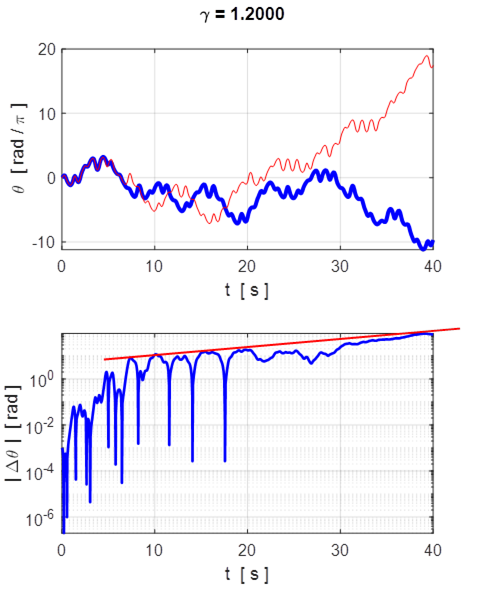
Fig. 9.3 Logarithmic plot of ![]() ,
the separation of two identical DDPs with a strong
driving force
,
the separation of two identical DDPs with a strong
driving force ![]() that were released with an extremely
small difference in initial angular displacements
that were released with an extremely
small difference in initial angular displacements ![]() .
The
motion for the large excitation initially shows that the two motions are almost
identical then suddenly they diverge as
.
The
motion for the large excitation initially shows that the two motions are almost
identical then suddenly they diverge as ![]() increases rapidly and irregularly with
time. Hence, the motions of the two pendulums diverge from one another with
time.
increases rapidly and irregularly with
time. Hence, the motions of the two pendulums diverge from one another with
time.
For the first few drive cycles, the two
pendulums move with very similar trajectories then the crests shown in figure 9.3
increase linearly, showing that ![]() increases
exponentially for some time. So, for chaotic damped driven motion of the
pendulum, we simple do not know where the pendulum will be in the future, since
even for minute differences in the initial conditions it will lead to
trajectories that are very different.
increases
exponentially for some time. So, for chaotic damped driven motion of the
pendulum, we simple do not know where the pendulum will be in the future, since
even for minute differences in the initial conditions it will lead to
trajectories that are very different.
The mean line drawn (red) to the logarithmic scale in ![]() implies
implies ![]() ,
hence
,
hence
![]()
where the parameter ![]() is known
as the Lyapunov
exponent. The above results for pendulums which start with nearly
identical initial conditions indicate that for small or medium forcing, the
motions will converge exponentially
is known
as the Lyapunov
exponent. The above results for pendulums which start with nearly
identical initial conditions indicate that for small or medium forcing, the
motions will converge exponentially ![]() whereas for high
forcing, the trajectories diverge exponentially
whereas for high
forcing, the trajectories diverge exponentially ![]() . The pendulum system while obeying
deterministic laws may still exhibit irregular and unpredictable behaviour due
to an extreme sensitivity to initial conditions.
. The pendulum system while obeying
deterministic laws may still exhibit irregular and unpredictable behaviour due
to an extreme sensitivity to initial conditions.
Chaotic motion exhibits extreme
sensitivity to initial conditions and it is this sensitivity makes accurate
predicts impossible.
10 Large
drive strengths
atmDDP.m
So far, we have observed the changes in
motion of the damped driven pendulum as we have increased the drive strength ![]()
Small ![]() linear
regime – pure sinusoidal
linear
regime – pure sinusoidal
Moderate ![]() nearly linear regime – addition of harmonics, subharmonics, period cascading
nearly linear regime – addition of harmonics, subharmonics, period cascading
Large ![]() nonlinear
regime – chaotic motion
nonlinear
regime – chaotic motion
But happens when we increase
drive strength further ???
We get another surprising result - the
motion is again periodic, but there is a drift along with the oscillation. For ![]() as shown
in figure (10.1), the pendulum is oscillating but also
consistently rotating all the way around until it reverses its direction of
rotations at irregular intervals. The phase space plot shows a series of almost
closed orbits and the general drift in the angular displacement.
as shown
in figure (10.1), the pendulum is oscillating but also
consistently rotating all the way around until it reverses its direction of
rotations at irregular intervals. The phase space plot shows a series of almost
closed orbits and the general drift in the angular displacement.
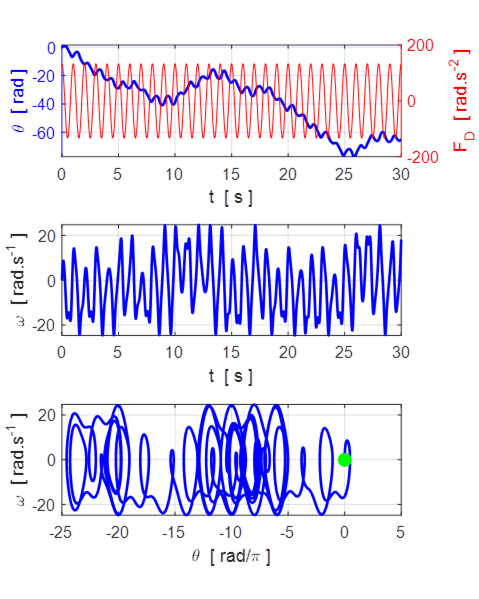
Fig. 10.1 Large
drive strength ![]() .
.
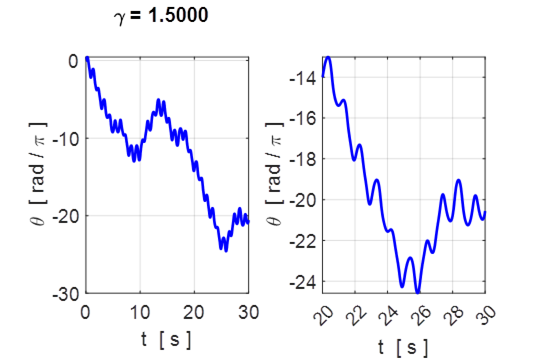
Fig. 10.2 Large
drive strength ![]() . Expanded view of the angular displacement
showing the erratic superimposed oscillations at the driving frequency as the
pendulum rotates.
. Expanded view of the angular displacement
showing the erratic superimposed oscillations at the driving frequency as the
pendulum rotates.
For the motion for ![]() as shown in figure 10.1, during the first
8 s the pendulum rotates anticlockwise approximately through 13 revolutions and
then starts to rotate in the other sense and again reverses direction around 15
s and 25. The pattern of movement never repeats itself. The motion can be
described as a rolling motion as the pendulum swings approximately through 2
as shown in figure 10.1, during the first
8 s the pendulum rotates anticlockwise approximately through 13 revolutions and
then starts to rotate in the other sense and again reverses direction around 15
s and 25. The pattern of movement never repeats itself. The motion can be
described as a rolling motion as the pendulum swings approximately through 2![]() (1
revolution) each drive cycle. The motion is chaotic. This chaotic motion is
emphasized in the phase space plot in figure 10.2 as the orbit fails to repeat
itself or to close o itself.
(1
revolution) each drive cycle. The motion is chaotic. This chaotic motion is
emphasized in the phase space plot in figure 10.2 as the orbit fails to repeat
itself or to close o itself.
If we decrease drive strength slightly to ![]() as shown
in figure 10.3 the motion is periodic with the angular velocity
as shown
in figure 10.3 the motion is periodic with the angular velocity ![]() returning to the same value once each
cycle.
returning to the same value once each
cycle.
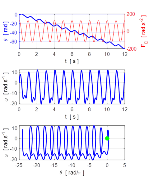
Fig. 10.3 Large drive strength ![]() . The motion is periodic with the angular
displacement
. The motion is periodic with the angular
displacement ![]() decreasing
2
decreasing
2![]() rad each
drive cycle. The angular velocity
rad each
drive cycle. The angular velocity ![]() is clearly periodic with period equal to
the drive period of 1 s.
is clearly periodic with period equal to
the drive period of 1 s.
The DDP executes a
“rolling” motion, making a complete a clockwise revolution each
drive cycle. The motion is again periodic with ![]() decreasing
by 2
decreasing
by 2![]() each
drive cycle.
each
drive cycle.
You will that that ![]() increases (figures 10.4 and
10.5) the DDP
actually alternatives between intervals of chaotic motion separated by
intervals of nonchaotic – periodic motion.
increases (figures 10.4 and
10.5) the DDP
actually alternatives between intervals of chaotic motion separated by
intervals of nonchaotic – periodic motion.
![]()
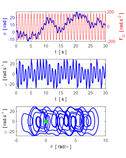
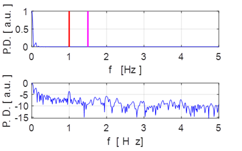
Fig. 10.4 ![]() Chaotic motion. Superimposed
on the drift in the angular displacement are the erratic oscillations at the
drive frequency of 1 Hz.
Chaotic motion. Superimposed
on the drift in the angular displacement are the erratic oscillations at the
drive frequency of 1 Hz.
![]()
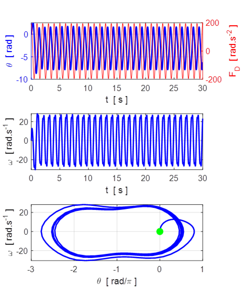
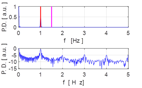
Fig. 10.5 ![]() Periodic motion. Note: strong fundamental
frequency (1 Hz) and prominent harmonics 2 (2 Hz), 3 (3 Hz), and 4 (4 Hz).
Periodic motion. Note: strong fundamental
frequency (1 Hz) and prominent harmonics 2 (2 Hz), 3 (3 Hz), and 4 (4 Hz).
The damped driven pendulum system is so-so
simple, but the response is anything but simple. As the amplitude of the
driving signal is increased, the motion changes from periodic to chaotic to
periodic with drift. This complex response is typical of nonlinear systems. The
motion of the pendulum for different model parameters is perplexing considering
the fact that the system is completely deterministic but with irregular
behaviour.
11 BIFURCATION
DIAGRAM
atmPendulumBDS.m
atmPendulumBD.m
The purpose
of a bifurcation diagram is to show in a single plot, the changing periods,
alternating periodicity, and chaos as the drive strength ![]() varies. It is a plot of
varies. It is a plot of ![]() or
a plot of
or
a plot of ![]() . Figure 11.1 shows the bifurcation diagrams
from Taylor’s book Classical Dynamics.
. Figure 11.1 shows the bifurcation diagrams
from Taylor’s book Classical Dynamics.
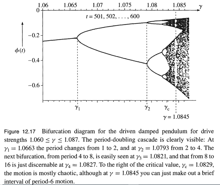
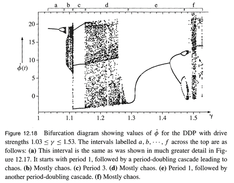
Fig. 11.1 Bifurcation diagrams from
Taylor’s book Classical Mechanics.
It is not an easy task to plot the
bifurcation diagram. The required
steps are:
1
Choose a large number of evenly spaced
values for ![]() from
from ![]() to
to ![]() .
.
2
Choose the initial conditions ![]() and
and ![]() .
.
3
Solve the equation of motion for DDP given by equation (1) for each value of ![]() for t =
0 to t = tmax.
for t =
0 to t = tmax.
4
Check for periodicity or non-periodicity
when all the transience has disappeared by examining ![]() or
or ![]() from
tmin to tmax
in one-cycle intervals with period T
from
tmin to tmax
in one-cycle intervals with period T
![]()
5
Plot these values of ![]() or
or ![]() from
tmin to tmax
against each value of
from
tmin to tmax
against each value of ![]() . For
larger values of
. For
larger values of ![]() the pendulum can start to make many
revolutions, so it is necessary to restrict
the pendulum can start to make many
revolutions, so it is necessary to restrict ![]() to the range
to the range ![]() . This can be done using the Matlab
statement X = atan2(tan(X),1) where X is the Matlab variable for
. This can be done using the Matlab
statement X = atan2(tan(X),1) where X is the Matlab variable for ![]() .
.
Fig. 11.2 shows the bifurcation diagrams of
the angular displacement ![]() and the
angular velocity
and the
angular velocity ![]() verses
the drive strength
verses
the drive strength ![]() . The bifurcation diagram is very
dependent upon choice of parameters and initial conditions. The diagrams show
the period doubling cascade effect. The angular displacement plot shown figure
11.2 is “poor” compared with Taylor’s plot shown in figure
11.1. Don’t know why the two diagrams are so
different in quality. Someone can have a look at my code and improve the Script
atmPendulumBDS.m.
. The bifurcation diagram is very
dependent upon choice of parameters and initial conditions. The diagrams show
the period doubling cascade effect. The angular displacement plot shown figure
11.2 is “poor” compared with Taylor’s plot shown in figure
11.1. Don’t know why the two diagrams are so
different in quality. Someone can have a look at my code and improve the Script
atmPendulumBDS.m.
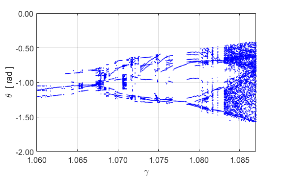
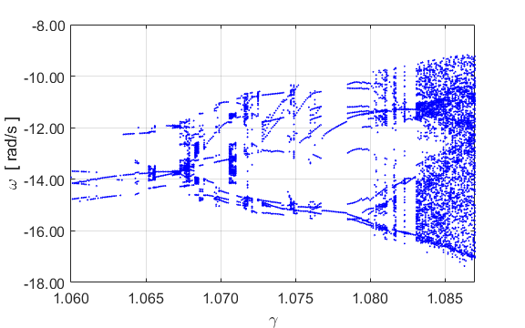
Fig. 11.2 Bifurcation diagrams for DDP. atmPendulumBDS.m
Figure 11.3 shows the plot ![]() which
shows the period doubling. So, an alternative way to construct the bifurcation
diagram is the find the peaks in the angular displacement
which
shows the period doubling. So, an alternative way to construct the bifurcation
diagram is the find the peaks in the angular displacement ![]() after the
transient oscillations have fully decayed for each value of the drive strength.
after the
transient oscillations have fully decayed for each value of the drive strength.
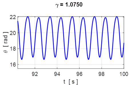
Fig.
11.3 Period doubling occurs
for ![]() since alternate peaks vary in
height. atmDDP.m
since alternate peaks vary in
height. atmDDP.m
Figure 11.4 shows the bifurcation diagram
constructed by finding the peaks in the angular displacement using the Matlab
function findpeaks.
The section of the Script atmPendulumBD.m that solves the ODE and finds the peak
values is
% Solutions X and w stored as a [2D] array
for k = 1 : Lgamma
K(3) = gamma(k)*wN^2;
[t, sol] = ode45(@(t,s) EM(t,s,K), tSpan,s0);
% Angular displacement and Velocity
X = sol(:,1);
w = sol(:,2);
% Find peak values
[a,
b] = findpeaks(X(tL-10000:tL),t(tL-10000:tL));
pks(k,:) = a;
% Restrict angular displacement to range -pi
to +pi
pks
= atan2(tan(pks),1);
end
The bifurcation diagram in figure 11.4 is an
improvement in the plot shown in figure 11.2. Period doubling from 1 to 2
occurs around ![]() ;
2 to 4 around
;
2 to 4 around ![]() ; 4 to 8 not resolved; and chaos when
; 4 to 8 not resolved; and chaos when ![]() . The details in figure 11.4 and much less
distinct than in Taylor’s plot shown in figure 11.1.
. The details in figure 11.4 and much less
distinct than in Taylor’s plot shown in figure 11.1.
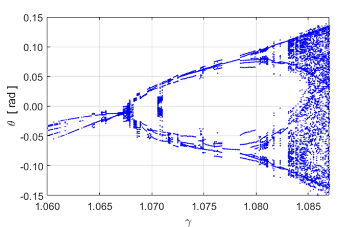
Fig. 11.4 Bifurcation diagram constructed by
find the peaks in the angular displacement after the transient oscillations
have fully decayed. It took
73 seconds for Matlab to perform all the operation to output . atmPendulumBD.m
Figure 11.5 shows bifurcation plots for a
larger range of drive strengths. Again, my plots are not well defined as
Taylor’s plot in figure 11.1. But, figure 11.5 shows a number of
transitions between periodic motion and chaotic motion.
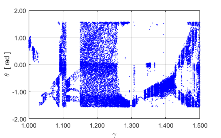
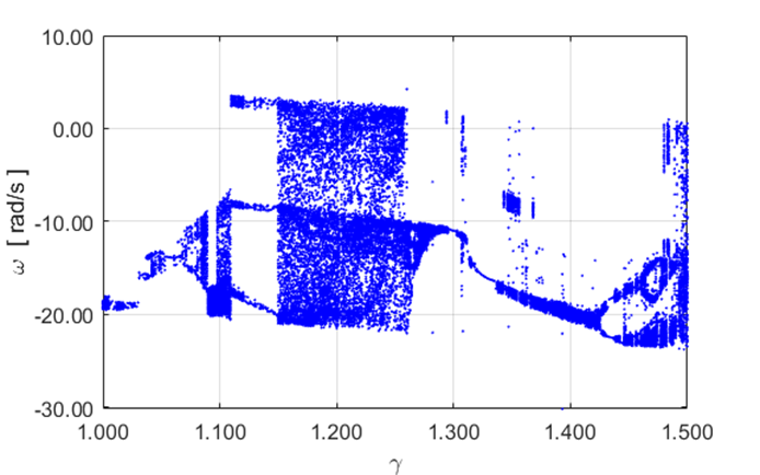
Fig. 11.5 Bifurcation diagrams for drive strength
![]() from 1.000 to 1.500. The Script atmPendulumBDS.m was used.
The Script atmPendulumBD.m could not be used because for
from 1.000 to 1.500. The Script atmPendulumBDS.m was used.
The Script atmPendulumBD.m could not be used because for ![]() the
pendulum motion became chaotic and no peaks can be identified using the
function findpeaks.
the
pendulum motion became chaotic and no peaks can be identified using the
function findpeaks.
12 POINCARE
SECTION
atmPendulumPS.m
There is a way to study chaotic motion that
is better than simply plotting the trajectory in phase space because after many
cycles it contains too much information to be useful. Consider the phase space
plot where points are not plotted at every time step but only at times given by
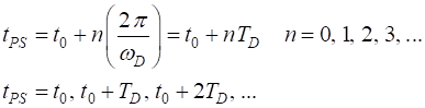
Such a phase space plot is called a Poincare
section. If the pendulum oscillates at the driving frequency, then
only one point will appear motion in the Poincare section. If the oscillation
has twice the frequency of the driving force, then the Poincare section will
have two points. If the motion is not periodic and chaotic the Poincare section
will consist of a pattern of points called the attractor. The attractor has a
structure that is frequently beautiful even though the motion unpredictable and
chaotic, yet at the same time preserve a coherent global structure.
Period 1 oscillations ![]()
For ![]() the motion is
periodic with the period equal to the drive period (1.00 s).
the motion is
periodic with the period equal to the drive period (1.00 s).
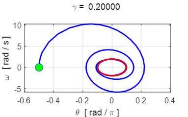
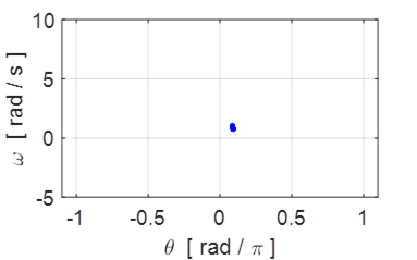
Fig. 12.1 The phase plot (red: orbit after transient motion decayed away) and
Poincare section for ![]() . Because the oscillation is described as period
1 motion, there is only one dot in the Poincare section.
. Because the oscillation is described as period
1 motion, there is only one dot in the Poincare section.
However, if you zoom in on the Poincare
section, there is a line of distinct points as shown in figure 12.2.
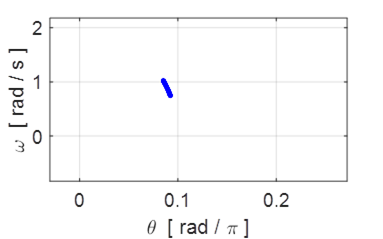
Fig. 12.2 The Poincare section shows a line
of points in the expanded view of figure 12.1 instead of a single point. WHY !!!
Period 2 oscillations ![]()
For ![]() the motion is
periodic with the period equal to twice drive period (1.00 s).
the motion is
periodic with the period equal to twice drive period (1.00 s).
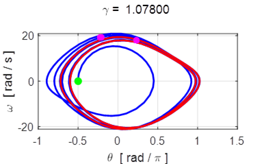
Fig. 12.3 The phase space plot for the DDP system ![]() . The red trajectory shows
the orbit for the last 100 time steps. The motion is period 2 since there are
two loops that make up one period of the oscillation. The magenta dots show the point that are displayed on
the Poincare section.
. The red trajectory shows
the orbit for the last 100 time steps. The motion is period 2 since there are
two loops that make up one period of the oscillation. The magenta dots show the point that are displayed on
the Poincare section.
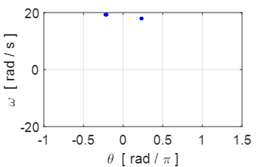
Fig. 12.4 Poincare section ![]() . The two points shown in the Poincare section
indicate the motion is period 2.
. The two points shown in the Poincare section
indicate the motion is period 2.
Next, we can look at the Poincare section
for chaotic motion. In Taylor’s Classical Mechanics his simulation
produced the plot shown in figure 12.5.
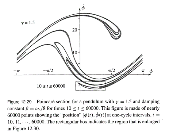
Fig. 12.5 Taylor’s Poincare section
for chaotic motion.
I could not reproduce the curves shown
in figure 12.5 using the same parameters as Taylor. ??? My plot is shown in figure 12.6.
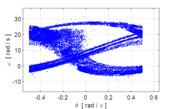
Fig. 12.6 Poincare section for chaotic
motion using the Script atmPenulumPS.m.
REFERENCES
Basic of
Atmospheric Science A. Chandrasekar
Classical
Mechanics J.R. Taylor
Collection of notebooks on dynamical systems http://www2.me.rochester.edu/courses/ME406/webexamp5/
http://galileoandeinstein.phys.virginia.edu/7010/CM_22a_Period_Doubling_Chaos.html
https://www.cfm.brown.edu/people/dobrush/am34/live/part3.html
Oscillations in Damped Driven Pendulum: A Chaotic System
https://www.arcjournals.org/pdfs/ijsimr/v3-i10/5.pdf