|
DYNAMICS OF
OSCILLATING AND CHAOTIC SYSTEMS SIMULATIONS:
DUFFING OSCILLATOR Ian Cooper matlabvisualphysics@gmail.om DOWNLOAD
DIRECTORY FOR MATLAB SCRIPTS chaos01.m
Runga-Kutta method for solving the equation of motion for a Duffing
oscillating: free, viscous damping and forced motions. chaos02.m
Runga-Kutta method for solving the equation of motion for a Duffing
oscillating: Poincare sections INTRODUCTION The
[1D] system we will simulate is a non-linear dynamical system described by
the equation of motion of a Duffing oscillator. The system of mass m is constrained to move only
along the X axis. The equation of motion can be expressed as (1) where x is the displacement of the system from the Origin c1 is the
damping coefficient c2 constant
where c2 > 0 c3 constant where c3 < 0 c4 is the
strength of the driving force c5 is the angular frequency of the driving force
angular driving frequency
period
The Duffing equation describes the motion of a
classical particle in a double well potential (figure 1). The
equation of motion (1) is solved using the Runge-Kutta
method to find the displacement x and velocity v at each successive time step
acceleration
net force
conservative force (free motion)
potential energy (conservative force)
potential
kinetic energy
total energy
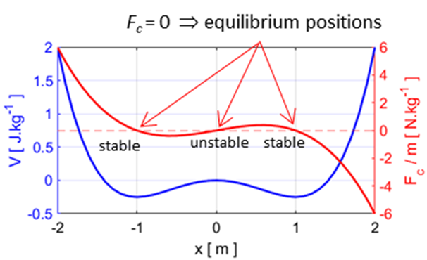
Figure
1 shows the displacement plots of the conservative force and its potential.
The potential is defined as the potential energy per unit mass (electric
potential is work per unit charge). To help understand and visualise a
Duffing oscillator, we can think of a particle of unit mass whose movement is
governed by the potential. Think of a [1D] marble rolling up and down hills and
valleys. The Duffing oscillator is equivalent to our marble between two
mountains with a small hill in the middle which separates to valleys. When
there is zero damping and no driving force, if the kinetic energy of the
“marble” is less than the potential energy at the top of the
hills, the marble will be trapped and will simple roll back and forth just as
a pendulum swings back and forth. The Duffing oscillator is like a marble
trapped forever in the region between the two mountains. The potential function
can be through of a two-well potential.
Fig.1.
Conservative force: potential and force curves as a function of
displacement for the case in which there is zero viscous damping and no
driving force The plots in figure 1 show that there
are three equilibrium at the points where At the bottom of two valleys.
For example, if the “marble” is given a small displacement from
the centre of a valley, the force acting on the marble will try to restore it
back to the equilibrium position. This is a stable equilibrium point. At the top of the small hill. If the “marble” is slightly displaced from the top
of the hill, the force is such that it will cause the marble to move further
way from the equilibrium point. This is an unstable equilibrium point. Because
of energy conservation one can clearly never get chaos from the motion of a
single degree of freedom. We therefore need to include both the driving force
and the damping in order to remove energy conservation. As the strength of
the driving force increases the motion of the classical particle becomes more
complicated and a transition to chaotic motion occurs. The
model of the double well potential we will use for all simulations is
and
the equation of motion is
where SIMULATIONS You
should do your own simulations by change the input parameters. Predict the
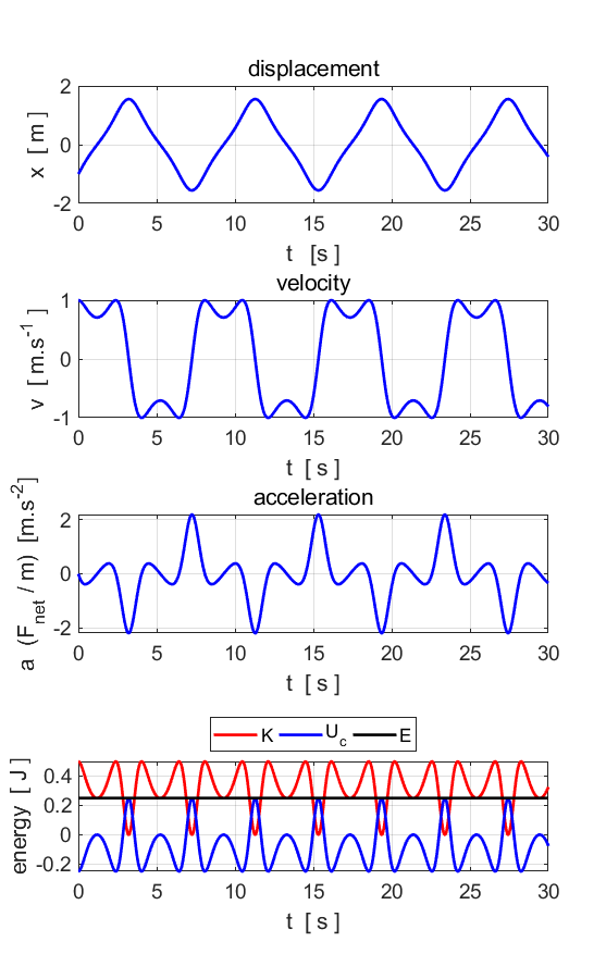
results and then run the script to test your predictions. Simulations #1 Free motion Zero
damping and no driving force Equation
of motion: We
will solve the equation of motion for our classical particle starting in the
left-hand minimum x = -1 with velocity equal to v = 1. This is big enough kick to get the particle over the hump in
the potential energy hill at x = 0 to the vicinity of the x = +1 minimum and back again. Why? (You should easily be able to
show from energy conservation that the particle will get over the hump if the
initial velocity is greater than Input
parameters c(1) = 0 c(4) = 0 c(5) = 0 m = 1.0 nT
= 1001 tMin = 0 tMax
= 30 x(1) = -1 v(1) = 1
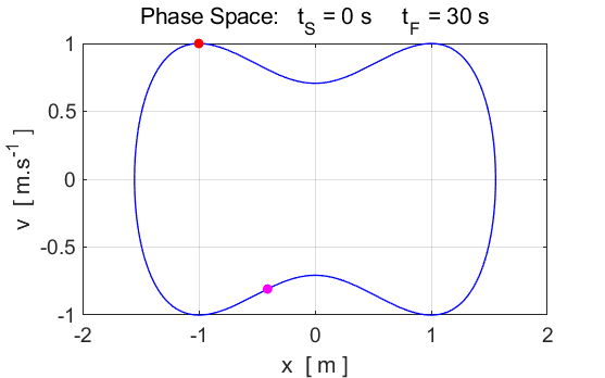
Fig. 2. The
motion of the oscillator is periodic. The attractor is the closed curve
(limit cycle) shown in the phase plot.
The total energy of the system is conserved as there are zero
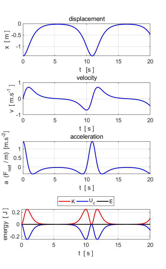
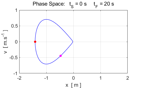
dissipative or driving force acting on the system. Simulations #2 Free motion: unstable equilibrium Zero
damping and no driving force Equation
of motion: Input
parameters c(1) = 0 c(2) = 1 c(3) = -1 c(4) = 0 c(5) = 0 m = 1.0 nT
= 1001 tMin = 0 tMax
= 20 x(1) = -1.414 v(1) = 0
Fig. 3. The
“marble” is launch from its starting position with zero kinetic
energy and zero potential energy. The marble falls into the valley and then
just reaches the top of the small hill which is an unstable equilibrium
point. The marble briefly stops at the top of the small hill before falling
back into the well. The motion of the marble is period as it rolls back and
forth in the valley. The phase plot shows the periodic nature of the
trajectory and the closed orbit and the attractor corresponds to the limit
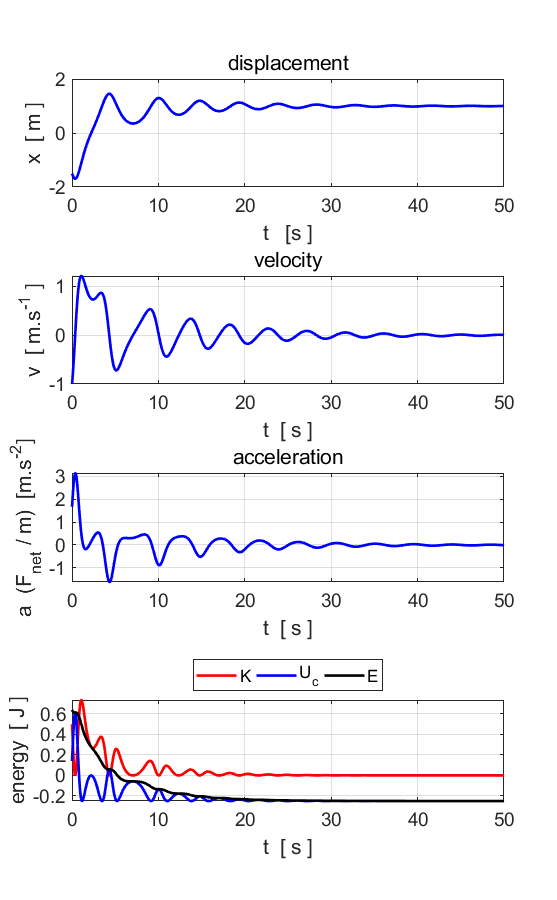
cycle. Simulations #3 Damped motion Damping
and no driving force Viscous damping
causes the oscillations to die-way. This is an example of a dissipative
system as energy is lost to the surrounding environment. Equation
of motion: Input
parameters c(2) = 1 c(3) = -1 c(4) = 0 c(5) = 0 Vary c(1) from 0 to 0.5 in
steps of 0.1 m = 1.0 nT
= 1001 tMin = 0 tMax
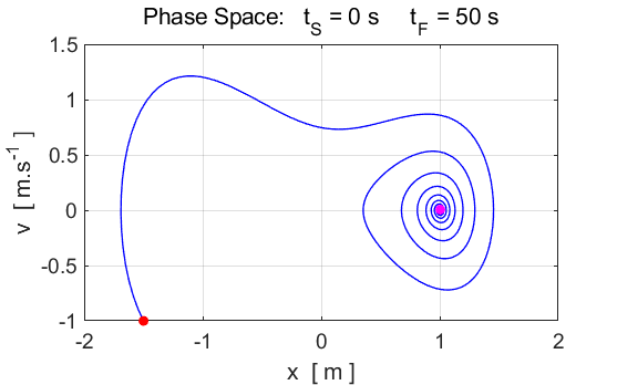
= 50 x(1) = -1.5 v(1) = -1.0
Fig.
5. The oscillations die-away.
There is a fixed point attractor at Simulation #4.1 Damped driven motion: The road to chaos Equation
of motion: When
a driving force acts upon the system, it increases the complexity of the
phase plots. When the strength of the driving force becomes large enough, the
motion of the particle becomes chaotic and is not possible to predict its
motion, since any slight changes in the model parameters results in a very
different movement of the particle. N.B. As the driving force strength increases you will need to
increase the maximum simulation time tMax and the
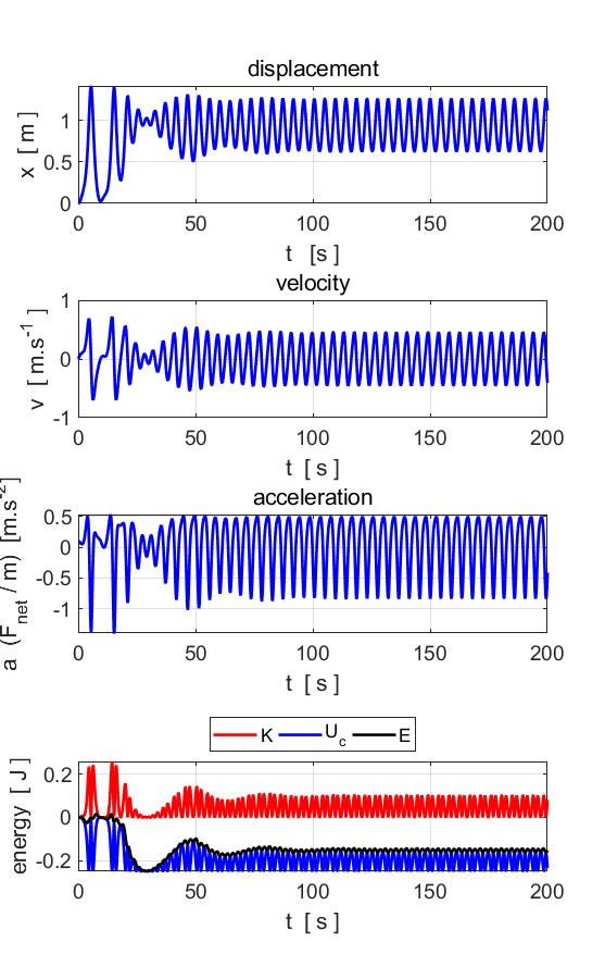
number of iterations nT Input
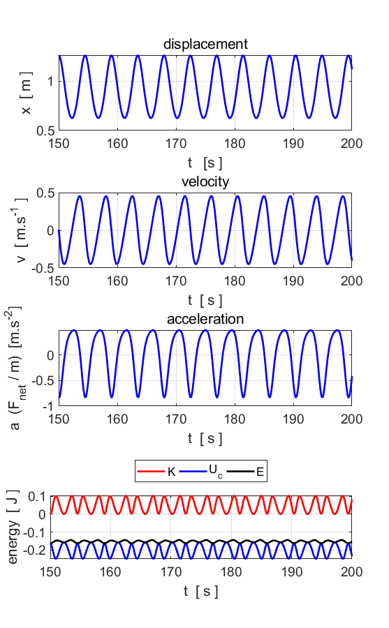
parameters c(1) = 0.1 c(2) = 1 c(3) = -1 c(4) = 0.1 c(5) = 1.4 m = 1.0 nT
= 1001 tMin = 0 tMax
= 200 x(1) = 0 v(1) = 0
Fig. 6A. After an initial transient behaviour, the particles
motion becomes periodic and oscillates at the driving frequency
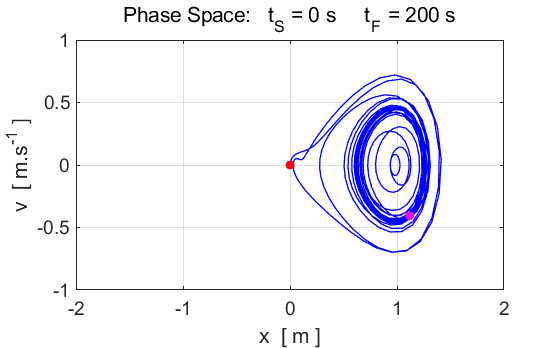
Fig. 6B. This
looks complicated, but in fact, most of the plot shows the initial period of
time during which the motion is approaching its final behaviour which is much
simpler. The early behaviour is called an "initial transient". To
see that this is the case, let's just look at the behaviour for t at later
times between 150 and 200 as shown in figure 6C.
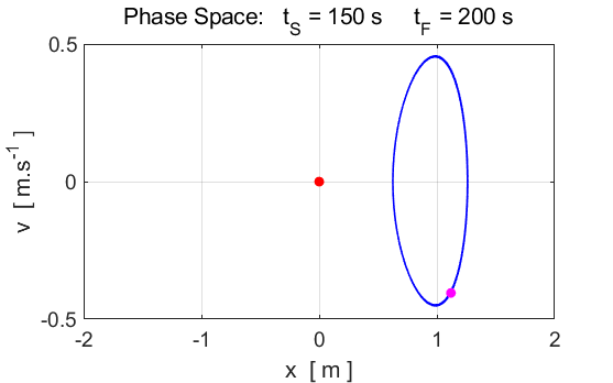
Fig.6C. After
some transient behaviour, the system stabilises, and the motion becomes
periodic. The period of oscillation is equal to oscillation of the driving
force. The phase space
trajectory encircles the fixed-point attractor (x = 1, v = 0) as it evolves to a closed orbit called the limit cycle. Simulation #4.2 Damped driven motion: The road to chaos
Equation
of motion: Increasing
the amplitude of the driving force (c4), a family of periodic orbits is obtained. However, as the
driving force increases further, the phase space trajectory begins to wander
away from the fixed-point attractor in a haphazard manner, but the motion is
not yet chaotic as shown in figure 7. If you watch the animation, you will
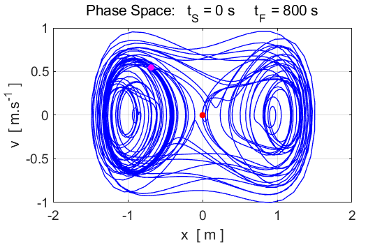
see the attraction of the system towards the three equilibrium fixed points. Input
parameters c(1) = 0.1 c(2) = 1 c(3) = -1 c(4) = 0.32 c(5)
= 1.4 m = 1.0 nT
= 1001 tMin = 0 tMax
= 800 x(1) = 0 v(1) = 0
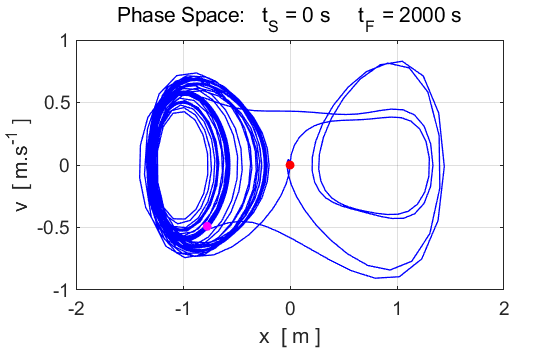
Fig. 7A. The
amplitude of the driving force is c4 = 0.32. The system wanders around between the fix-point
attractors at
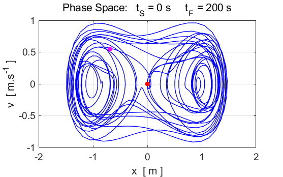
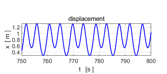
Fig. 7B. The
particle moves through both of the wells. However, again, most of this
complexity is due to an initial transient.
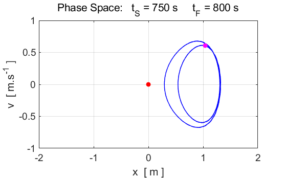
Fig. 7C. The
phase space plot becomes much simpler after the initial transient period. The
particle settles down near the x = +1 minimum, and once it has done so, goes
twice around x = +1, v = 0 before retracing its path. Depending on the exact
value of the strength of the damping force c(4) and the initial conditions,
the particle could also have gone into a doubled orbit near the x = -1
minimum. In fact, the period has doubled Simulation #4.3 Damped driven motion: The road to chaos Equation of
motion: A
further increase in the strength of the driving force can lead to a further period
doubling. Input
parameters c(1) = 0.1 c(2) = 1 c(3) = -1 c(4) = 0.34 c(5)
= 1.4 m = 1.0 nT = 8001 tMin
= 0 tMax = 2000 x(1) = 0 v(1) = 0
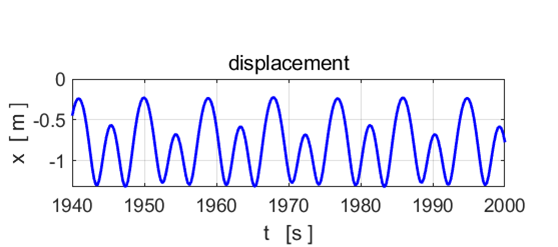
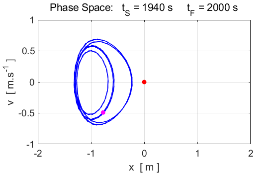
Fig. 8. The
orbit now goes 4 times round the point x = -1 before repeating. The period
has doubled again Simulations #4.4 Damped driven motion: The road to chaos Equation of
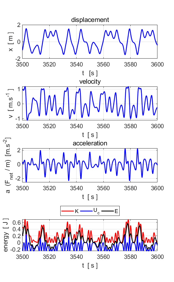
motion: Further
increasing the amplitude of the driving force leads to chaotic motion. The phase
space trajectory wanders around in a more or less aimlessly manner. Slight
changes in the initial conditions leads to very different phase space
trajectories. Hence, the trajectory becomes unpredictable. Input
parameters c(1) = 0.1 c(2) = 1 c(3) = -1 c(4) = 0.38 c(5)
= 1.4 m = 1.0 nT = 18001 tMin
= 0 tMax = 3600 x(1) = 0 v(1) = 0
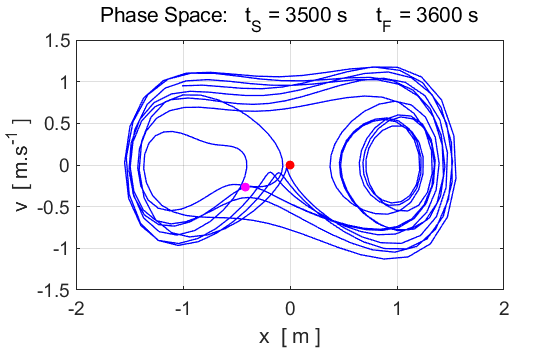
Fig.
9. The motion does not settle
into a periodic orbit. The motion of the particle is now chaotic. POINCARE SECTIONS There
is a way to study chaotic motion that
is better than watching a trajectory wander around in phase space. For a
system which includes the viscous damping and an externally applied driving
force, the Poincare
section is constructed on the
phase plot (x vs v graph) by only plotting points every If
the orbit in phase space is periodic, with this period, then we will get only
one point displayed on the plot. If the orbit has a period equal to two times
the period of the driving force, then the Poincare section will show two
points, and so on. If the system is chaotic, the Poincare section will
consist of a pattern of points called the attractor. The attractor has a
structure that is often beautiful. A surprising result is that a
deterministic system can exhibit unpredictability and apparent chaos and at
the same time preserve a coherent global structure. Simulations #5 Poincare
sections
chaos02.m A
useful way of analysing chaotic motion is to look at what is called the
Poincare section. Rather than considering the phase space trajectory for all
times, which gives a continuous curve, the Poincare section is just the
discrete set of phase space points of the particle at every period of the
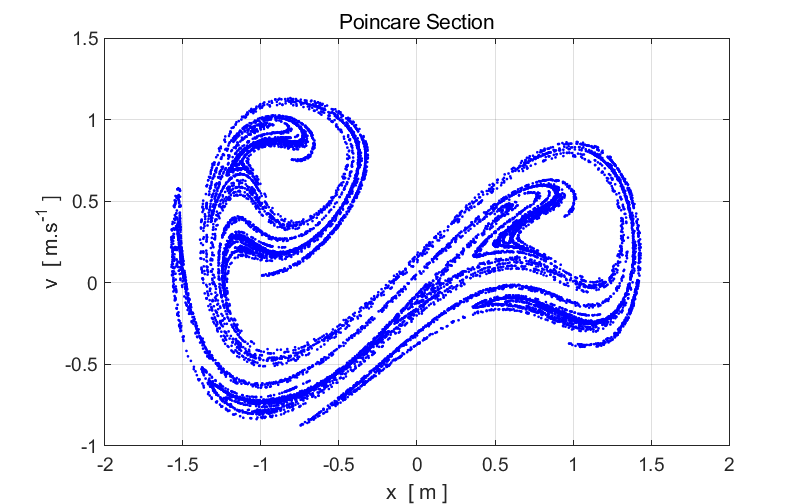
driving force, i.e. at Input
parameters c(1) = 0.1 c(2) = 1 c(3) = -1 c(4) = 0.38 c(5) = 1.4 m = 1.0 nT
= 501 nP
= 18000 x(1) = 0 v(1) = 0 nT is the
number of calculations before another point is plotted. nP is the
number of points pointed at time intervals of For
figure 10, nP =18000, which is a very large number.
nP must be large enough to plot enough points to
show the structure of the Poincare section. It took about 3 minutes to
calculate and plot the Poincare section.
Fig. 10. Poincare section of the Duffing two-well oscillator.
This strange diagram is the strange attractor. It is the limiting set of
points to which the trajectory tends to after every time interval equal to
the period of the driving force. Notice that the structure is complicated but
not completely random. We see structure.
|