|
DYNAMICS OF
OSCILLATING AND CHAOTIC SYSTEMS POINCARE SECTIONS:
DUFFING OSCILLATOR Ian Cooper matlabvisualphysics@gmail.com DOWNLOAD
DIRECTORY FOR MATLAB SCRIPTS chaos02.m Runga-Kutta method for solving the equation of motion for a Duffing
oscillating with viscous damping and forced motions. Computation for the
Poincare section for a phase space plot. All parameters are changed within
the script. chaos01.m
Runga-Kutta method for solving the equation of motion for a Duffing
oscillating: free, viscous damping and forced motions: time; displacement;
and phase space plots. All parameters are changed within the script.
Animations of the trajectories are saved as animated gif files. The script
could be altered so the animations are saved as avi
files. POINCARE SECTIONS There
is a way to study chaotic motion that
is better than watching a trajectory wander around in phase space. For a
system which includes the viscous damping and an externally applied driving
force, the Poincare
section is constructed on the
phase plot (x vs v graph) by only plotting points every If
the orbit in phase space is periodic, with this period, then we will get only
one point displayed on the plot. If the orbit has a period equal to two times
the period of the driving force, then the Poincare section will show two
points, and so on. If the system is chaotic, the Poincare section will
consist of a pattern of points called the attractor. The attractor has a
structure that is often beautiful. A surprising result is that a
deterministic system can exhibit unpredictability and apparent chaos and at
the same time preserve a coherent global structure. Simulations
#1 Poincare
sections
chaos02.m A
useful way of analysing chaotic motion is to look at what is called the Poincare
section. Rather than considering the phase space trajectory for
all times, which gives a continuous curve, the Poincare section is just the
discrete set of phase space points of the particle at every period of the
driving force, i.e. at Input
parameters c(1) = 0.1 c(2) = 1 c(3) = -1 c(4) = 0.38 c(5) = 1.4 m = 1.0 nT
= 501 nP
= 24000 nS
= 1 x(1) = 0 v(1) = 0 nT is the
number of calculations before another point is plotted. nP is the
number of points plotted at time intervals of nS is the
start number for plotting the points. For
figure 1, nP =24000, which is a very large number. nP must be large enough to plot enough points to show the
structure of the Poincare section. It took about 4 minutes to calculate and
plot the Poincare section.
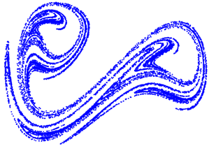
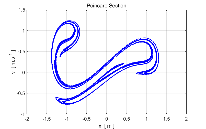
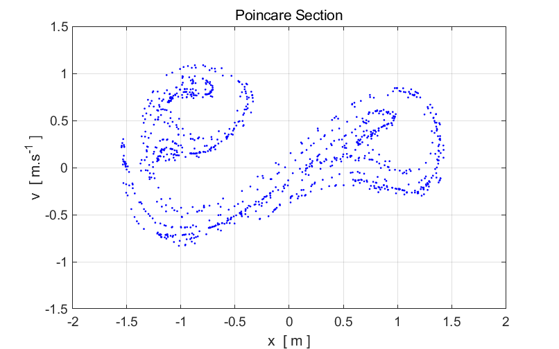
Fig. 1.
Poincare section of the Duffing two-well oscillator. This strange diagram is the strange attractor. It is the limiting set of
points to which the trajectory tends to after every period of the driving
force (after the initial transient). Notice the that the structure is
complicated but not completely random, we see structure. The
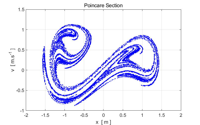
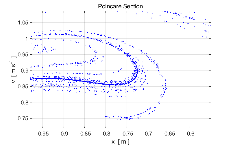
Fractal Nature of Chaotic Attractors The
structure of a Poincare section can be viewed in more detail by using the Zoom In
button in the Figure Window. When you Zoom In it
will take some time for the screen to update because of the large number of
points that are plotted. Zoom In on a small region of the strange
attractor and examine its structure. Zoom In again and view the structure of
the strange attractor. You will notice that the features of the strange
attractor at the smaller scale are similar to those features at the larger
scale – there appears to be a fine structure. Having the same features appearing in different parts of a
figure and at different scales is a characteristic feature of a fractal.
An attractor
is fractal
if a set of points that shows self-similarity as the scale being used
decreases. In practice, you cannot keep zooming in, because fewer and fewer
points will be displayed and if you keep increasing the number of points, the
computation time becomes very large.
Fig. 2. Expanded
views of the Poincare section displayed in figure 1 for the two-well Duffing
oscillator. Simulations
#2 Poincare
sections
chaos02.m Input
parameters c(1) = 0.24 c(2) = 1 c(3) = -1 c(4) = 0.88 c(5) = 1.7 m = 1.0 nT
= 501 nP
= 24000 x(1) = 1 v(1) = -1
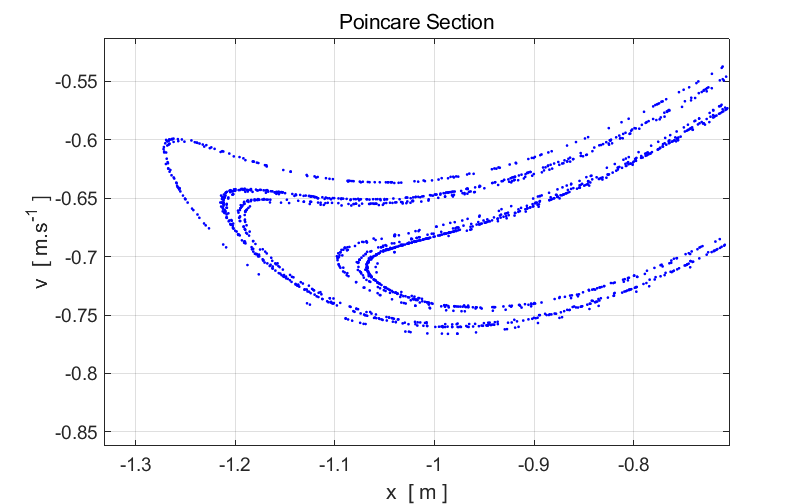
Fig.
3. Poincare section of the
Duffing two-well oscillator and an expanded view of the lower left portion of
the attractor. Note the structure that emerges. Simulations
#3 Poincare
sections – period doubling: the road to chaos chaos02.m Input
parameters c(1) = 0.10 c(2) = 1 c(3) = -1 c(4) = 0.1 c(5)
= 1.4 m = 1.0 nT
= 501 nP
= 4000 nS = 3000 x(1) = 0 v(1) = 0
Fig. 4. The
period of the oscillator is T. The Duffing oscillator oscillates at the driving frequency.
Hence, the driving period is equal to the period of the oscillation. Only one
point is displayed in the Poincare section.
View
chaos01, simulation #4.1 Fig. 6. Input
parameters c(1) = 0.10 c(2) = 1 c(3) = -1 c(4) = 0.32 c(5) = 1.4 m = 1.0 nT
= 501 nP
= 4000 nS = 3000 x(1) = 0 v(1) = 0
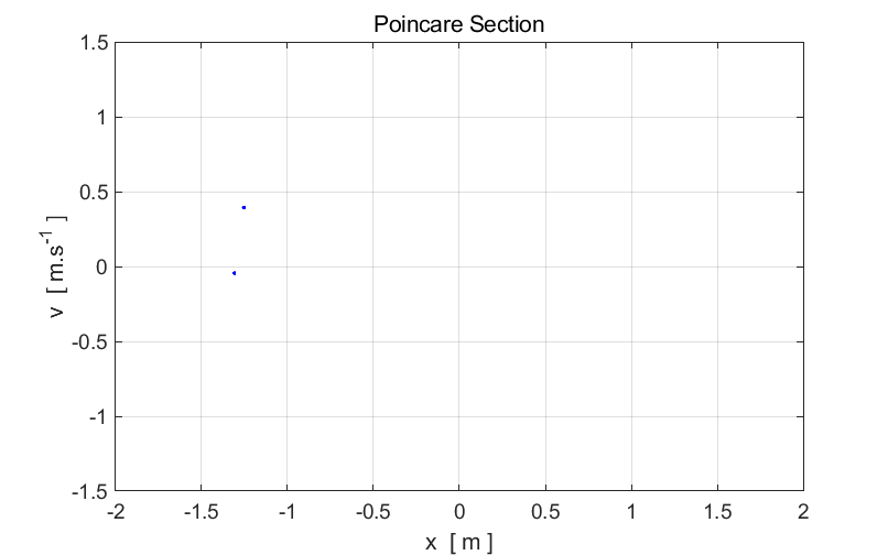
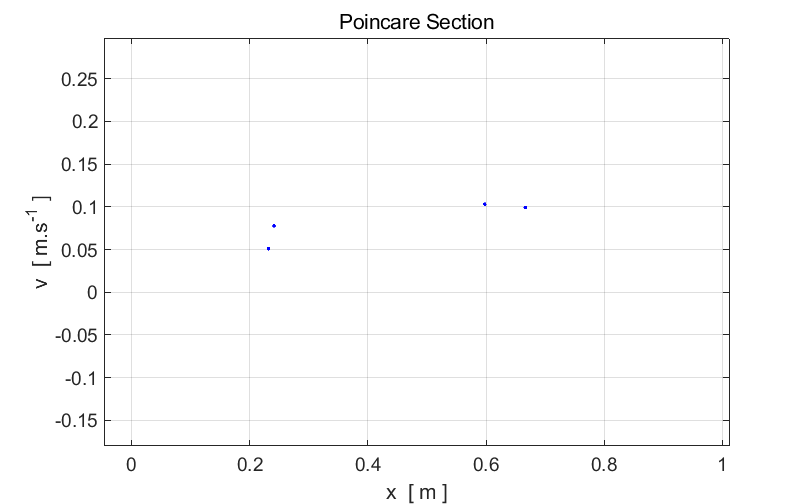
Fig. 5. The
period T of
the Duffing oscillator is now twice the period of the driving force
View
chaos01, simulation #4.2 Fig. 7. Input
parameters c(1) = 0.10 c(2) = 1 c(3) = -1 c(4) = 0.34 c(5) = 1.4 m = 1.0 nT
= 501 nP
= 4000 nS = 3000 x(1) = 0 v(1) = 0
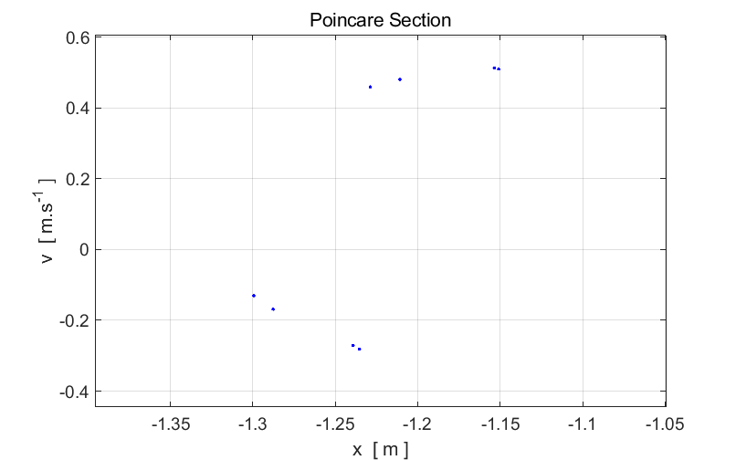
Fig. 6.
Expanded view. The period T of the Duffing oscillator is now four times the period of the
driving force
View
chaos01, simulation #4.3 Fig. 8. Input
parameters c(1) = 0.10 c(2) = 1 c(3) = -1 c(4) = 0.3425 c(5) = 1.4 m = 1.0 nT
= 501 nP
= 4000 nS = 3000 x(1) = 0 v(1) = 0
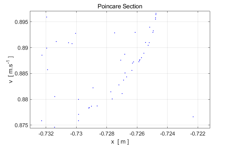
Fig. 6.
Expanded view. The period T of the Duffing oscillator is now eight times the period of the
driving force
Input
parameters c(1) = 0.10 c(2) = 1 c(3) = -1 c(4) = 0.35 c(5) = 1.4 m = 1.0 nT
= 501 nP
= 4000 nS = 3000 x(1) = 0 v(1) = 0
Fig. 5. The
motion is no longer periodic – the motion has become chaotic. Note: the slight change in the strength of the diving force
given by the variable c(4) results in a transition
from periodic
motion to chaotic motion.
Logistic
maps can produce fractal patterns. Integrating a differential equation
requires much more time than iterating a logistic map. Therefore, people have
investigated maps which have similar behaviour to that of driven, damped
differential equations like the Duffing equation. Thus, we can come to a quite an exciting conclusion – the beautiful world of fractals tentatively touches the fascinating field of chaotic dynamics.
|