|
DYNAMICS OF
OSCILLATING AND CHAOTIC SYSTEMS RIGID PENDULUM Ian Cooper matlabvisualphysics@gmail.com DOWNLOAD
DIRECTORY FOR MATLAB SCRIPTS chaos07A.m
Runga-Kutta
method for solving the equation of motion for a rigid pendulum with damping
and applied external driving force acting on the system. chaos07AB A
bifurcation
diagram for the driven damped
pendulum. INTRODUCTION The
system we will simulate is a rigid pendulum where a mass m is attached to a rigid massless rod so that the centre of mass
is a distance L from a
frictionless pivot. There is viscous damping of the motion and an externally applied sinusoidal driving force acting on
the pendulum. The system is constrained to move in a plane. The net force
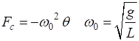
acting on the system is the resultant force due to the gravitational force The
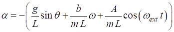
equation of motion of this system is governed by the equation of motion (1) where
(2a)
(2b)
where
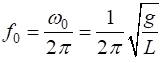
oscillations
angular frequency
natural frequency
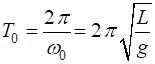
period
This
system is called a non-linear dynamical system since the
differential equation describing the system contains non-linear terms. Equation
2 is the equation of motion that is solved using the Runge-Kutta
method. The
Matlab variables for the angular displacement, angular velocity and angular
acceleration are: In
the Matlab script chaos07A.m the
equation of motion (equation 2) is given in terms of the global variable c which is a matrix of four elements. The differential
equation (equation 2) is given by the Matlab function % Equation of motion function y = fn(t,x,v) global c y =
- ( c(1)*sin(x) + c(2)*v + c(3)*cos(c(4)*t) ) ; end The default value for the parameters:
m, g, T0, L, c(1) are specified in the CONSTANTS and
DEFAULT section of the script chaos07A.m. The
INPUT section of the script chaos07A.m is used to
set the values: nT
number of time steps tMax
simulation time tS and
tF
start and finish times for displaying the graphical output c(2), c(3) and c(4) differential
equation coefficients x(1) and v(1)
initial values for angular displacement and angular velocity The
Runga-Kutta algorithm computes the angular
displacement and angular velocity at each time step. Then the angular
acceleration, kinetic energy, potential energy and total of the energy of the
system are calculated.
acceleration
restoring force
kinetic energy
potential energy (conservative force
total energy
potential
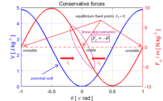
We
can define a potential
function V associated
with the conservative force FC acting on the system. The potential V is the potential energy per unit mass (electric potential is the
work done per unit charge).
Fig. 1. Conservative force and
associated potential curve for the rigid pendulum. The
conservative force acting on the pendulum is such that it is in a direction
to try and restore the pendulum to its equilibrium position at There
are two equilibrium positions for the pendulum. These two equilibrium points
are called fixed
points in chaotic dynamics. The
two fixed points are: 1.
When the
pendulum is hanging down from its pivot point 2.
When the
pendulum is standing directly above the pivot point. This is an unstable equilibrium
point. SIMULATIONS chaos07A.m Simulation #1 Small amplitude, free motion of the rigid
pendulum For small amplitude oscillations, the
motion of the pendulum bob is to a good approximation described by the
equations of simple harmonic motion with a natural period of oscillation The
default value for all simulations is Input parameters
nT = 801 tMax
= 5 tS = 0 tF
= t(end)
c(2) = 0
c(3) = 0
c(4) = 0
zero damping and zero applied force
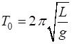
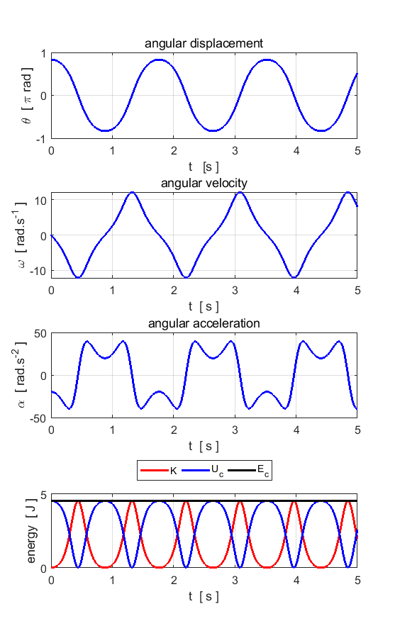
x(1) = Graphical outputs
Fig. 1.1. The motion of the pendulum bob
is to a good approximation simple harmonic motion with a period of ~1.0 s.
The total energy is conserved. The
potential curve (figure 1) is approximately a parabolic function of angle for
small angular displacements,
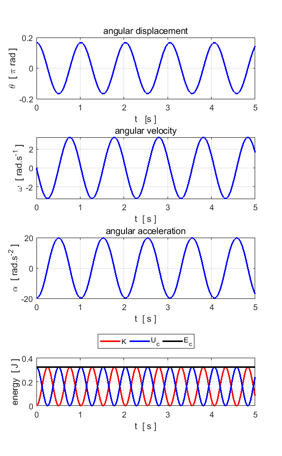
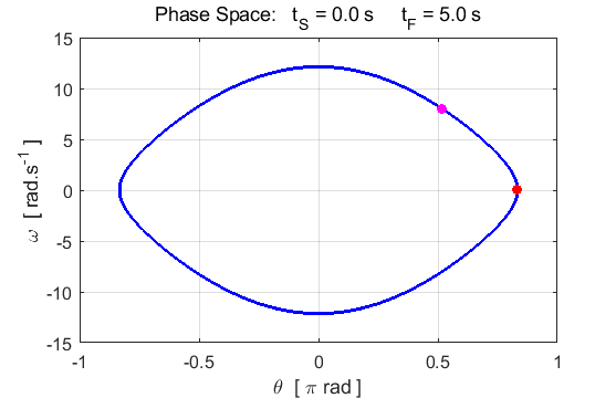
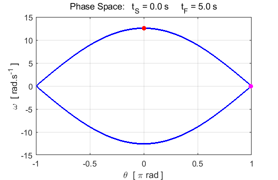
Fig. 1.2. The
phase space diagram for simple harmonic motion is an ellipse. The red dot shows the
initial position of the pendulum bob and the magenta dot, the final position.
After 5 periods, the pendulum does not return to its initial starting
position. Therefore, the motion is not truly simple harmonic motion. If you
make the initial angular displacement smaller, then the better the
approximation to simple harmonic motion.
Fig. 1.3.
Animated motion of the pendulum and its phase space plot. Simulation #2 Large amplitude, free motion of the rigid
pendulum For large amplitude oscillations, the
motion of the pendulum bob is no longer executing simple harmonic motion.
However, the motion is still periodic. Input parameters
nT = 801 tMax
= 5 tS = 1 tF
= t(end)
c(2) = 0
c(3) = 0
c(4) = 0
zero damping and zero applied force
x(1) = 5 Graphical outputs
Fig. 2.1. Large amplitude oscillations.
The pendulum is no longer executing simple harmonic motion. The motion
however is still periodic. The period is now longer
Fig. 2.2. Phase space portrait for the motion of
the pendulum. The trajectory forms a closed loop which is called the limit
cycle. The closed loop indicates that the motion of the pendulum is periodic.
Fig. 2.3. Animated motion of the pendulum
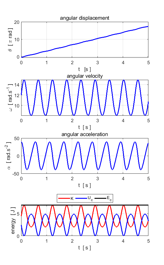
in phase space. Simulation #3
Free rotation of the pendulum The
pendulum is given an initial push so that is continually rotates in an
anticlockwise sense Input parameters
nT = 801 tMax
= 5 tS = 0 tF
= t(end)
c(2) = 0
c(3) = 0
c(4) = 0 zero damping and zero
applied force
x(1) = - Graphical outputs
Fig. 3.1. The pendulum spins in
anticlockwise sense.
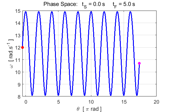
Fig. 3.2. Phase space portrait.
Fig. 3.3. Animated motion of the spinning
pendulum. There is no orbit for the phase
plot – the phase space curve is an open one. Simulation #4
Unstable equilibrium The
pendulum starts at the bottom of its swing in the stable equilibrium fixed
point. The pendulum is given an initial velocity so that the pendulum will
swing to a point vertically above the pivot point. This point is an unstable fixed
equilibrium point. The pendulum hovers at the unstable equilibrium
fixed point momentarily before falling. How big a push do we need? The
initial velocity can be estimated from the principle of conservation of
energy Initial total energy
at the bottom of the swing
Final total energy at the bottom
of the swing
Energy is conserved Initial angular velocity
Input parameters
nT = 801 tMax
= 5 tS = 0 tF
= t(end)
c(2) = 0
c(3) = 0
c(4) = 0
zero damping and zero applied force
x(1) = 0
v(1) = 12.566
initial angular displacement and angular velocity Graphical outputs
Fig. 4.1. The pendulum comes to rest momentarily
at the unstable equilibrium fixed point directly above the pivot before
falling.
Fig. 4.2. Phase space plot is a closed loop
(limit cycle) indicating a periodic orbit.
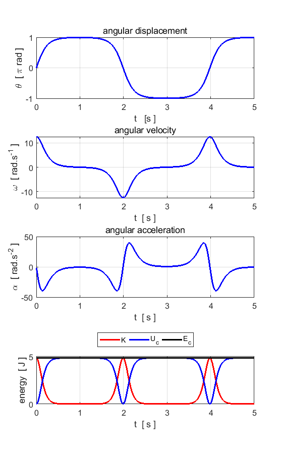
Fig. 4.3. Animation of the phase space plot. Simulation #5
Damped motion The
phase
space plot is a very important
one to help you visualize the behaviour of our system and to understand
chaotic dynamics. The viscous damping causes the pendulum to slow down as
energy is dissipated and lost to the surroundings. The behaviour of the pendulum slowing
down, and the motion attracted to a fixed equilibrium point is illustrated
very well in a phase space plot. The simulations for damped motion have the
same initial conditions use in Simulation #3 (free rotation). Increasing the
magnitude of the variable c(2) increasing the
damping of the system. Try different simulations by increasing the value of c(2). Before running a simulation, predict the behaviour
of the system and then test your predictions Input parameters
nT = 801 tMax
= 5 tS = 0 tF
= t(end)
c(2) = 1 c(3) = 0 c(4) = 0
zero applied force
x(1) = Graphical outputs
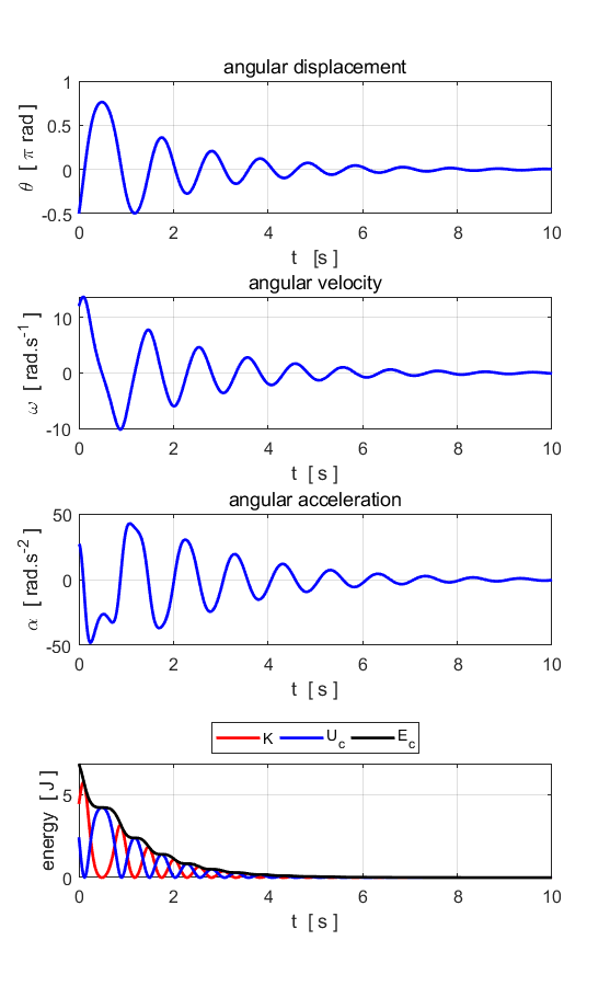
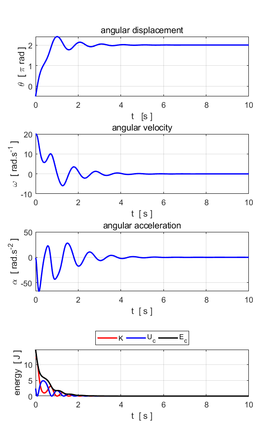
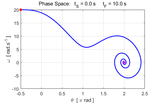
Fig. 5.1. The motion of a damped pendulum.
Energy is dissipated and lost to the surroundings. In
the above plots, the pendulum swings with a decreasing amplitude until is
stops at the fixed point
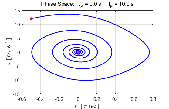
Fig. 5.2. Animated motion of the damped
pendulum. Input parameters increased damping
nT = 801 tMax
= 5 tS = 0 tF
= t(end)
c(2) = 2 c(3) = 0 c(4) = 0
zero applied force
x(1) = Graphical outputs
Fig. 5.3. Strong damping causes the
oscillations to quickly die-away. The
attractor at
the fixed point in phase space is
Fig. 5.4. Animation of the damped motion
of the pendulum. Simulation #6
Forced damped motion: RESONANCE One
can study the phenomenon of resonance when a damping force and external
driving force act upon the system. The damping force causes the dissipation
of energy from the system. However, an externally applied force may add or
subtract energy from the system. When the frequency of the driving force is
equal to the natural frequency of oscillation of the pendulum, then, maximum
energy can be transferred into the system by the externally applied driving
force. This results in the maximum amplitude of oscillation of the pendulum
(provided that the strength of the driving force is not too large). If the
driving frequency is not equal to the natural frequency, then the system will
oscillate at the frequency of the driving force with a
lower amplitude as a smaller net amount of energy is transferred to
the system. The greater the difference in the frequency of the driving force
and the natural frequency, then, the smaller the amplitude of pendulum
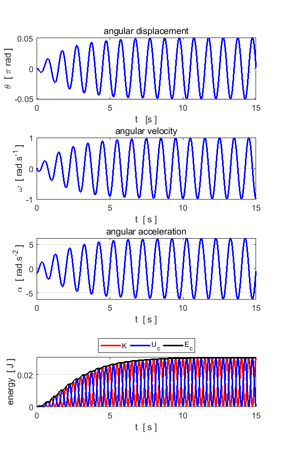
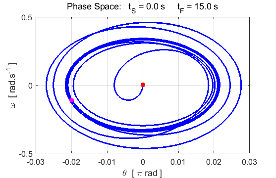
oscillation. Input parameters RESONANCE
nT = 801 tMax
= 15 tS = 0 tF
= t(end)
c(2) = 1 c(3) = 1
c(4) = 2*pi/T0 driving frequency =
natural frequency
x(1) = 0 v(1) = 0
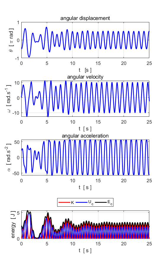
initial angular displacement and angular velocity Graphical outputs
Fig. 6.1. The applied external driving
force transfers energy to the pendulum while energy is lost from the system
because of the viscous damping force. After approximately 8 s the energy
dissipated and transferred to the system balance and then the total energy
remains constant and the pendulum swings back and forth in a periodic manner
with a period of 1.0 s (period of driving force = natural period of
oscillation).
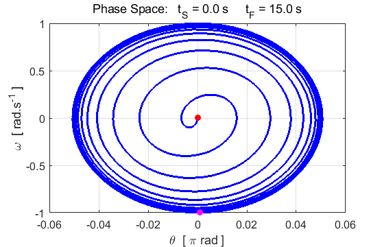
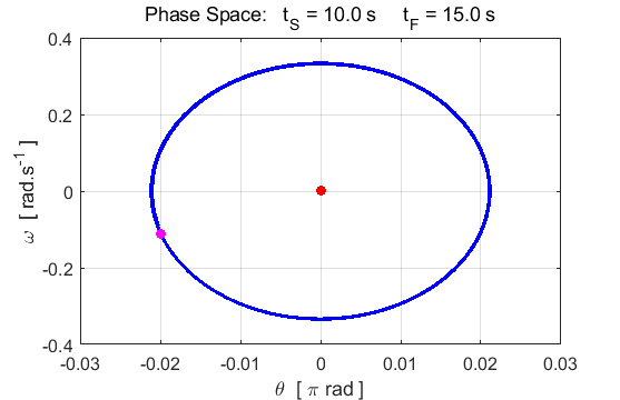
Fig. 6.2 The amplitude of the oscillation
increases until the amplitude reaches its maximum value. After about 8 s a
steady elliptical orbit is achieved in the phase space plot (nS = 8).
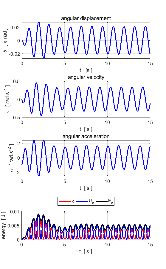
Fig. 6.3. Animation of the oscillating pendulum. Input parameters System not excited at its
natural frequency nT
= 801 tMax = 15 tS
= 0 tF = t(end)
c(2) = 1 c(3) = 1
c(4) = 0.8*2*pi/T0 driving frequency
< natural frequency
x(1) = 0 v(1) = 0
initial angular displacement and angular velocity Graphical outputs
Fig. 6.4. The driving frequency is less
than natural frequency. The pendulum swings with a smaller amplitude as less
energy is added to the system.
Fig. 6.5. The phase space plot is a very
useful way to illustrating important aspects of the motion. After some transient behaviour (~ 8 s), the system stabilizes.
The trajectory encircles the point
Fig. 6.6. Animation of the pendulum motion. Simulation #7
The road to chaos Adding
a driving force increases the complexity of the phase space plots. Small
changes in the strength of the driving force may result in very different
trajectories of the pendulum. It is not possible for the motion of the
pendulum to be chaotic if the forces acting of the pendulum are only the
gravitational force and the damping force. Chaos can only occur if an
external driving force also acts on the system and the driving frequency is
less than the natural frequency of oscillation When
the strength of the driving force exceeds a critical value, the motion
becomes chaotic
-the motion of the pendulum becomes erratic and unpredictable since very
small changes in any parameters such as time step, initial values results in
a very different trajectories. Model parameters Default values:
m = 1.0000 kg g =
9.8000 m.s-2
T0 = 1.0000 s à
w0 = 2*pi rad.s-1 = 6.2832 rad.s-1 f0 = 1.000 L = 0.2482 m
c(1) = 4*pi^2 = 39.4784
rad2.s-2 The
damping given by coefficient c(2) should not give
critical or overdamping, otherwise, the value used is not so important.
nT = 10000 tMax
= 25 tS = 0 tF
= t(end)
c(2) = 0.5 c(3) = 17
c(4) = 2*pi/T0 driving
frequency = natural frequency
x(1) = -pi/2
v(1) = 0 initial
angular displacement and angular velocity Graphical outputs
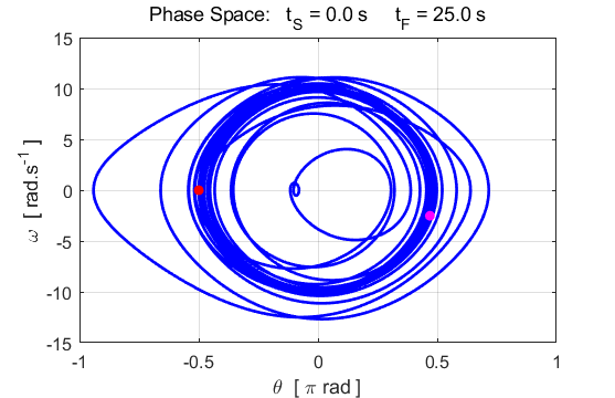
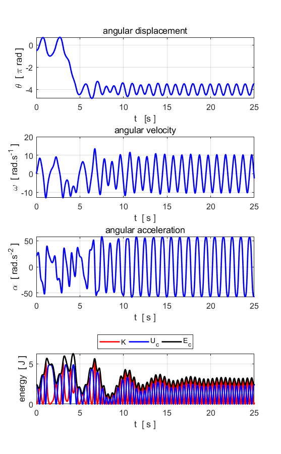
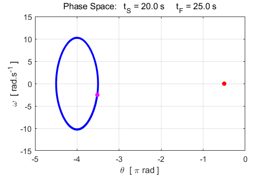
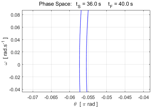
Fig. 7.1. For values of the strength of
the external driving force c(3) up to about 17, the angular displacement to a
good approximation is given by a sine curve and the phase space plot is an
ellipse (closed loop: limit cycle) with its centre at the fixed point
attractor The strength of the driving force c(3) increased slightly: 17 à
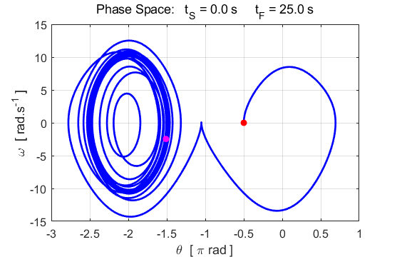
18. The
increase in the driving force causes the trajectory to wander in a haphazard
manner that appears to be chaotic but is not. The trajectory moves away from
the fixed-point attractor at
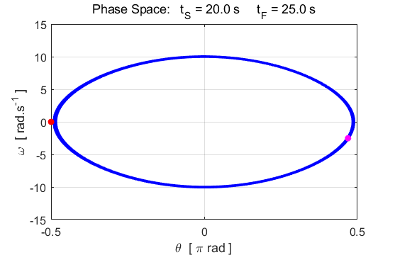
Fig. 7.2. The
motion of the pendulum for driving force strength c(3)
= 18. The motion becomes periodic around the fixed-point attractor
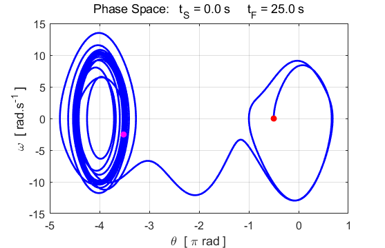
Fig. 7.3. c(3) = 19.
The pendulum motion stabilizers about the fix-point attractor
Input parameters: Driving frequency < natural
frequency
Increasing the strength of the
driving forces --> chaos
nT = 10000 tMax
= 40 tS = 0 tF
= t(end) c(2)
= 0.2 c(3) = 0
c(4) = 0.5*w0 driving
frequency < natural frequency
x(1) = -pi/2
v(1) = 0
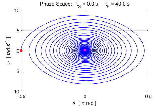
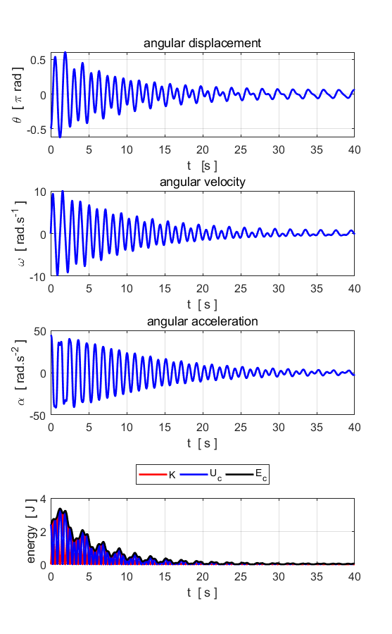
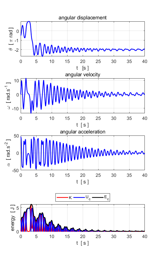
initial angular displacement and angular velocity Graphical outputs
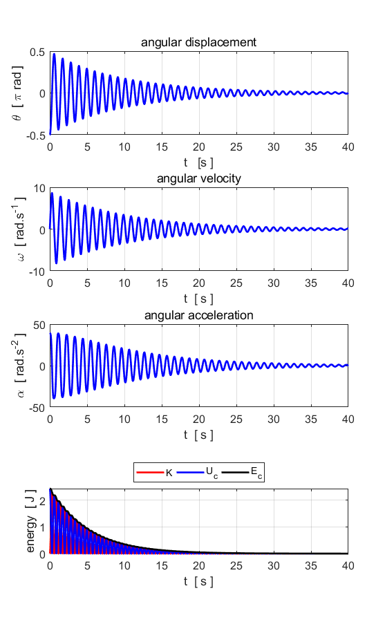
Fig. 7.5. c(3) = 0 Damped system with zero driving force. The oscillations die-away and the
pendulum comes to rest at the fixed-point attractor c(3)
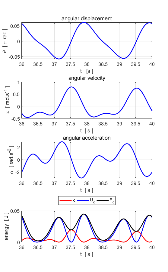
= 5
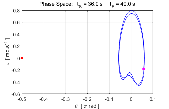
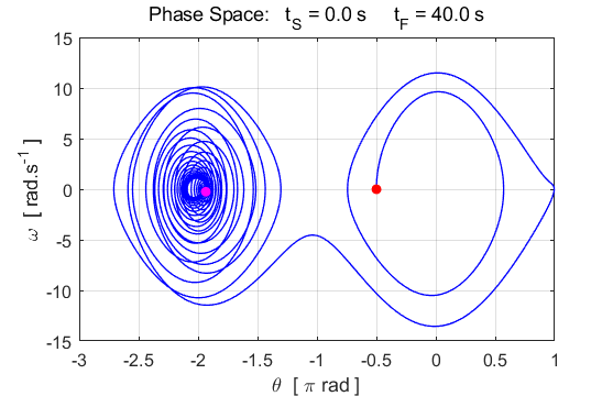
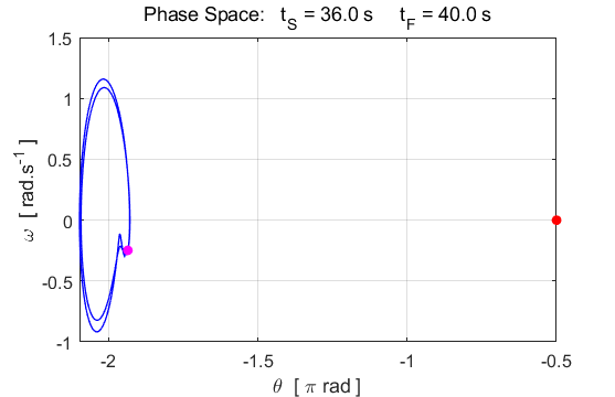
Fig. 7.5. c(3) = 5 The period of the oscillation is now 2.0 s, which is
double the period of the driving frequency TExt =
1.0 s. The doubling of the period is shown clearly by the double orbit in the
zoom phase space view (lowest plot). c(3) = 7
Fig. 7.6.
c(3) = 7 Periodic motion with a
2.0 s orbit around the fix-point attractor at c(3) = 15
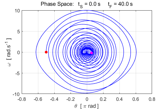
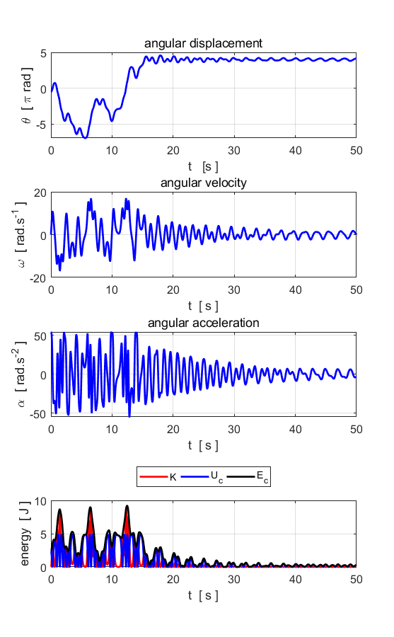
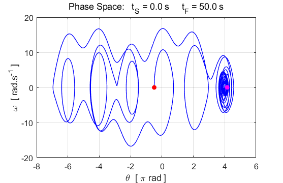
Fig. 7.7. c(3) = 15 The
motion of the pendulum is now chaotic.
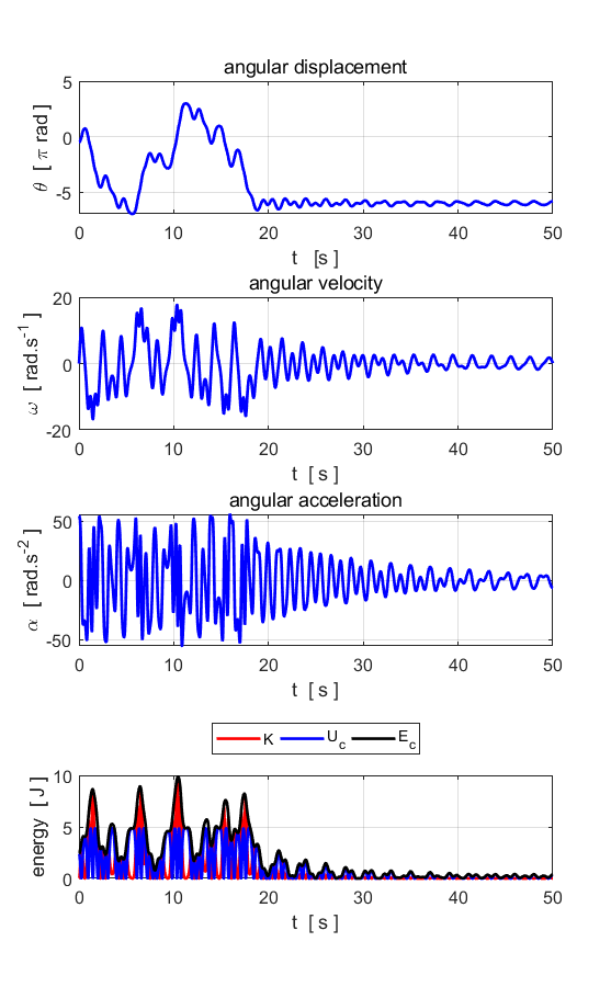
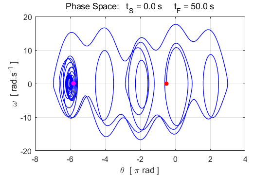
Fig. 7.7. c(3) = 15 v(1) = 0.001 The motion of the
pendulum is now chaotic. The slight increase in the initial angular velocity
(0.000 à 0.001) produces a very different
oscillation pattern.
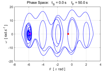
Fig. 7.7. c(3) = 15 The
chaotic motion of the pendulum is now chaotic. The motion is not predictable
since a slight change in initial values gives a very different trajectory. Left plot: v(1) = 0.000
and right plot: v(1) = 0.001. The motion is truly chaotic. When the motion of the pendulum has become chaotic,
the trajectory in phase space wanders about aimlessly, sometimes the pendulum
rotates clockwise and at other times it rotates anticlockwise about the pivot
point. It appears to be pulled towards one of the stable points, then wanders
away again to another attractor fixed point.
Fig.
7.8. Animated motion of the
chaotic pendulum for figure 7.6.
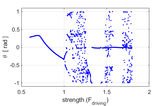
Simulation #8 BIFURCATION DIAGRAM A bifurcation diagram can be used to show
chaos. The script chaos07AB.m was used to give the
bifurcation diagram shown in figure 8. The parameters used for the
bifurcation are from Classical
Mechanics by J. R. Taylor
Fig.
8.1. Bifurcation diagram of
a driven damped pendulum. chaos07AB.m The diagram may
not be too good. Maybe there is a better way to get the bifurcation diagram. Input
parameters and Calculations: % INPUTS
=========================================================== % Time domain nT =
5000; % Max time interval tMax =
50;
tMin = 0;
t = linspace(tMin,tMax,nT);
h = t(2) - t(1); % Time interval for phase
space plot start tS and finsih
tF
% Iindices
nS and nF for plotting
figure 3 phase space plot tS =
0; tF =
t(end);
nS = find(t >= tS,1); nF
= find(t >= tF,1); nR = nS:nF; % nautral
frequency c(1) = 9*pi^2; % Damping constant c(2) = 3*pi/2; % Angular frequecny of driving force c(4) = 2*pi; % Initial position of
pendulum xA
[rad] vA
[rad/s]
x = zeros(nT,1);
v = zeros(nT,1); x(1) = 0; v(1) = 0.000; % Strength of driving
force c(3) = Fs*c1 % nS number
of calculations for varying strength of driving force % Fs strength of
driving force factor % theta angular displacent
at the end of the simulation %
-pi <= theta <= +pi nS =
2000; Fs = linspace(0.6,1.8,nS); theta = zeros(nS,1); % CALCULATIONS
======================================================== for cs
= 1 : nS c(3) = Fs(cs)*c(1); % Runga-Kutta
Solution of differential equation for cc = 1 : nT-1 [k1, k2,
k3, k4] = coeff(t(cc),h,x(cc),v(cc)); x(cc+1)
= x(cc) + h*(v(cc) + (k1 + k2 +k3)/6);
v(cc+1)
= v(cc) + (k1 + 2*k2 + 2*k3 + k4)/6; end theta(cs)
= x(end); while theta(cs) > +pi; theta(cs) =
theta(cs) - pi; end while theta(cs) < -pi; theta(cs) =
theta(cs) + pi; end end |