LORENZ
ATTRACTOR
Ian Cooper matlabvisualphysics@gmail.com DOWNLOAD
DIRECTORY FOR MATLAB SCRIPTS chaos23.m Lorenz
attractor: Trajectories and animations chaos23A.m Lorenz
attractor: global bifurcation diagram INTRODUCTION
In
this article, I will show how Matlab can be used to visualize the solution of
the Lorenz coupled ordinary differential equations for the Lorenz chaotic
attractor. This system of equations was first described by Edward Lorenz in
1963. He was a M.I.T. meteorologist and mathematician who was interested in
fluid flow models of the atmosphere. A
chaotic system is one that must show sensitivity to initial conditions, it
must be topologically
mixing, its orbits must be dense, and for a short time the solutions will be
nearly identical to one another and as time increases the trajectories of the
chaotic systems will suddenly have
no correlation with the other and solutions will diverge no matter how small
change is made to the initial conditions. The idea of topological mixing
implies that the system will evolve over time such that every open set of its
phase space will eventually intersect with every other open region. The
density of the orbits is also of importance to prove that a system is acting
chaotically. Orbits may never come close to anything resembling repeating
themselves. The
equations describing the Lorenz chaotic attractor are:
Parameters
The
most popular values for the parameters are:
x, y, z The
x and y parameters relate to the vertical and horizontal temperature variations
in the atmosphere respectively, and the z component is related to the
convection in atmospheric flow. x,
y, z all vary dynamically in time. x
is the convective flow (motion of heat through the atmosphere as hot air
rises), positive x pertains to clockwise motion. y
is the horizontal temperature distribution, found by taking the difference between
ascending and descending currents, positive y pertains to warmer currents on
the right (correlates strongly with positive x) z
is the vertical temperature distribution. For
some values of the three parameters Critical points (fixed points) There
are three fixed points, xC, yC, and zC
where the x, y and z parameters are constant
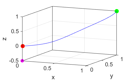
An
obvious critical point is the Origin (0, 0, 0). To find the other critical points, we
can take the yC component as a
free parameter such that
then
the other fixed points or critical points are
xC = yC and All
three fixed points are unstable.
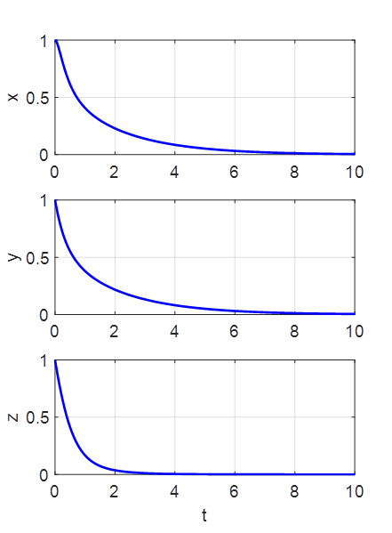
If the initial position corresponds to a fixed point, the values of x, y, and
z never change. However, even a small deviation in starting values from a
fixed point will cause the system to evolve so that the trajectory will
always be repelled from a fixed point if it tries to approach it. If The
system of the three coupled ordinary differential equations is solved using
the Matlab command ode45. The Script chaos23.m facilitates
simulations with the Lorenz equations. Model parameters are changed in the
INPUT section of the Script and the results are displayed in a series of
Figure Windows. Significance of Lorenz in Atmospheric Dynamics · Allows
us to see how different emissions spread by convection through the atmosphere.
· Allows
us to model weather and wind more accurately. · Allows
us to model the effect of anthropogenic emissions on vertical and horizontal
temperature gradients. SIMULATION
1 The
Script is run with two slightly different sets of initial conditions.
Initially the oscillations are very similar but after about 15 time-units,
the motions diverge and both become chaotic. Parameters: Initial
displacements blue
red
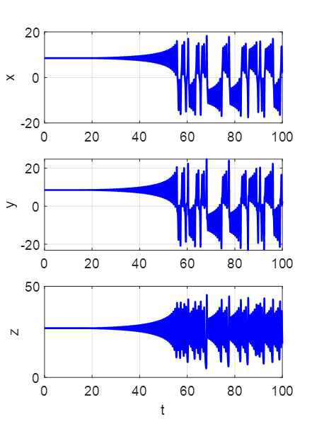
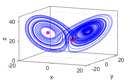
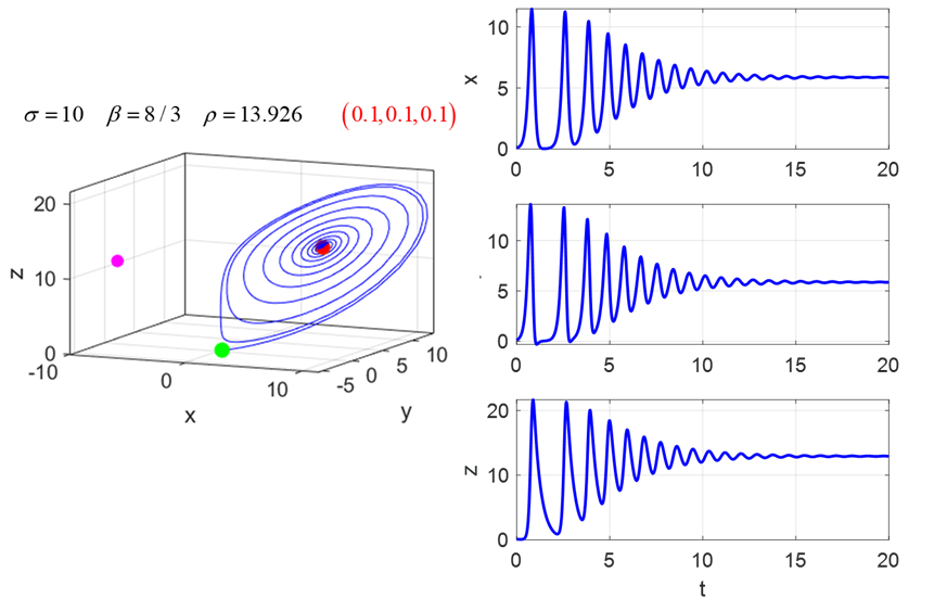
SIMULATION 2 The
initial displacement is set at the fixed point
x0 =
8.485281374238570 y0
=
8.485281374238570 z0
= 27 for
the parameters
For
a long period, the trajectory oscillates around the starting fixed point.
However, as the trajectory approaches this fixed point it is always repelled,
leading to chaotic motion as it later oscillates around the both of the fixed
points for ever. The trajectory is completely determined by the initial
starting position. The motion is not random but it is not predictable. SIMULATION
3 For
the parameters
SIMULATION
4 If
the Rayleigh number
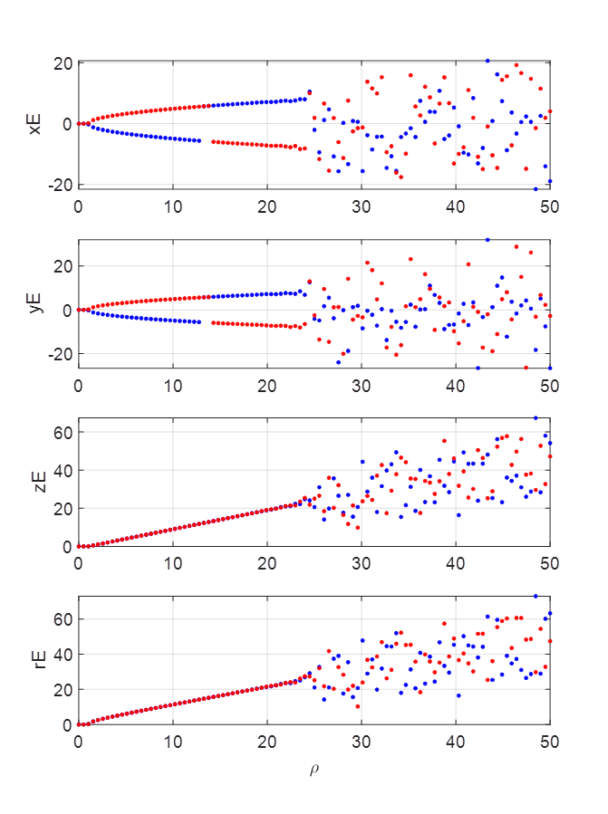
SIMULATION
5 Global bifurcations
Initial
conditions The
values xE, yE,
zE and Another
interesting behaviour is that there exists a homoclinic
bifurcation.
If
you start near the Origin and follow the unstable manifold trajectory outward,
you’ll eventually end up attracting to a limit cycle in one of the two
“lobes” when
REFERENCES https://www.youtube.com/watch?v=Q_f1vRLAENA |