|
Ian Cooper matlabvisualphysics@gmail.com DYNAMICAL
NON-LINEAR SYSTEMS LOGISTIC
DIFFERENCE EQUATION
DOWNLOAD DIRECTORIES FOR MATLAB
SCRIPTS chaosLogisticsEq01.m The logistic difference equation for the population chaosLogisticsEq02.m The logistic difference equation for the population chaosLogiscticsEq03.m Period doubling: plots of a [1D] mapping function f(n)(x) against the population x and the plot f(x) = x. The
intersections of the two curves gives the fixed points. For a fixed point to
be stable requires chaosLogisticsEq04.m Finding the fixed points for the population dynamics from a [1D] mapping function for different orders. INTRODUCTION Biologists studying the variability in populations of various species where generations do not overlap found a simple difference equation that predicted the population trajectories reasonably well. One such equation is a simple quadratic equation called the logistic difference equation. Very surprising, this simple difference equation predicts under certain circumstances a fantastically complex and chaotic behaviour that was total unexpected. The logistic difference equation is given by
where x(n) is a scaled population at iteration n and
r is the control or growth parameter. The initial condition is
specified by
This simple non-linear system does not possess simple
dynamical properties It
is often observed in nature that a population x
will increase from one generation to the next when small and decrease when
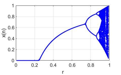
large. This is expressed mathematically by the product The population For small values of r, the population converges to a stable equilibrium population. As the value of r increases, interesting things happen as shown in figure 1.
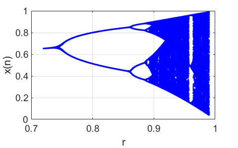
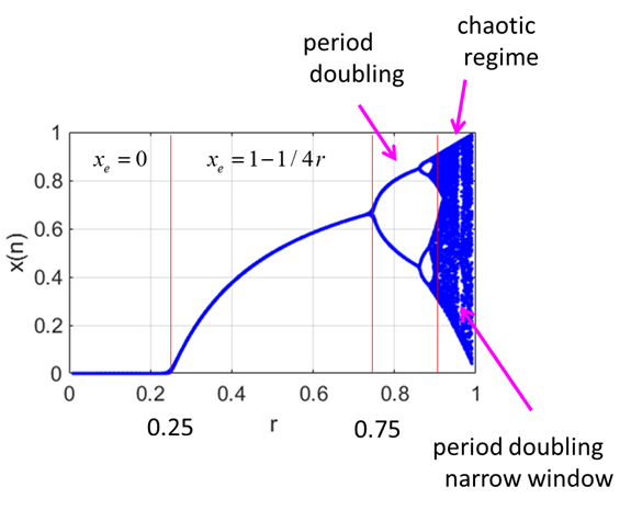
Fig.
1. Bifurcation diagram
- plot of the iterated values of of the growth parameter r. Note the transitions from stable equilibrium populations to oscillation and period doubling to chaotic behaviour and region of periodic behaviour within the region of chaos. chaosLogisticsEq01.m When r > ~0.75, Figure 2 show an animated plot of the iterated values of the population for increasing values of the growth parameter r. As r passes through one of its critical values, note the complete change in the dynamics of the system.
Fig. 2. Animated
plot of the iterated values of the population increasing values of the growth parameter r. chaosLogisticsEq01.m The quadratic expression in the logistic difference equation is
The function PERIOD 1
DYNAMICS
The orbit of the population x is attracted to an equilibrium
point or fixed point
One
obvious fixed point is
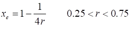
We
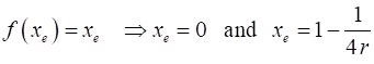
can derive analytical expressions for the fixed points of the [1D] map
Since
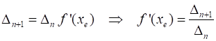
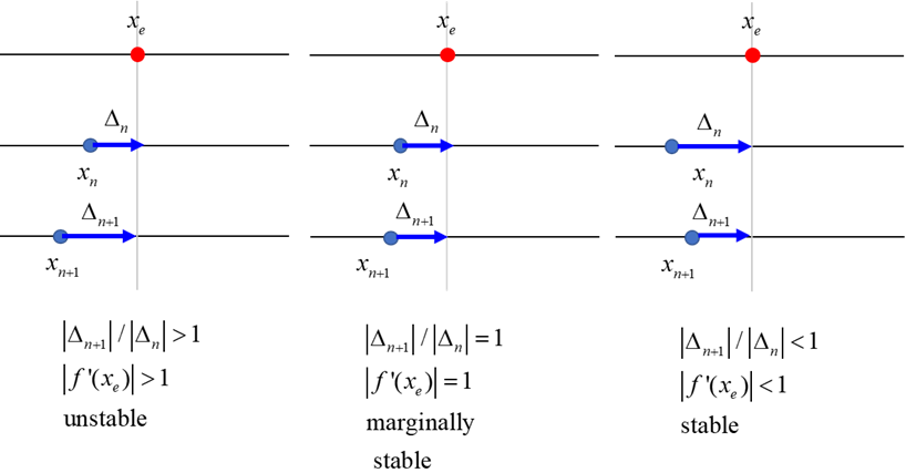
To determine the stability of the fixed points
and we have
If If Thus, the local stability criteria for a fixed point
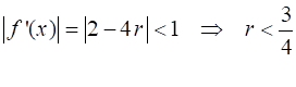
Fig 3. Stability of fixed points The first derivative is
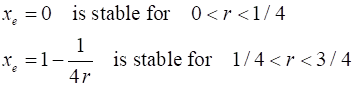
Thus, for the equilibrium point
Therefore, we can conclude
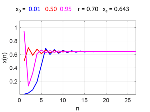
The local curvature of the curve Using the Script chaosLogisticsEq02.m you can explore the dynamical behaviour
of the system by inputting different values for the initial population
Fig. 4. Plots of the
iterated population initial populations x0 = 0.01, x0 = 0.50 and x0 = 0.95. The stable fixed
point is
This dynamic is said
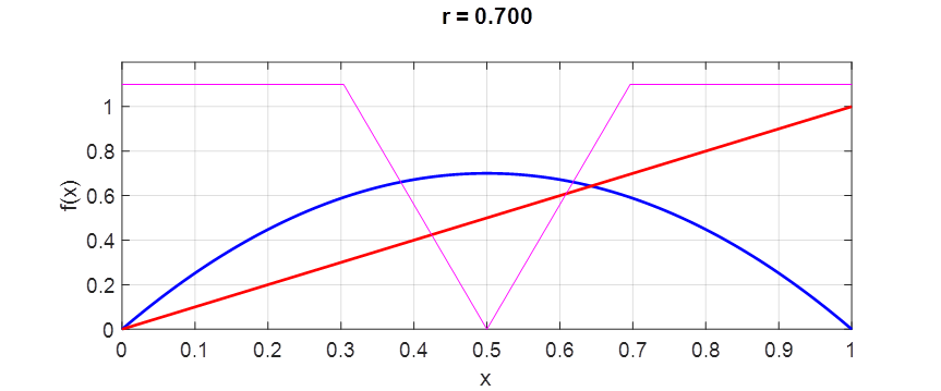
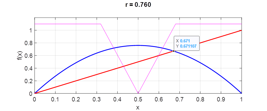
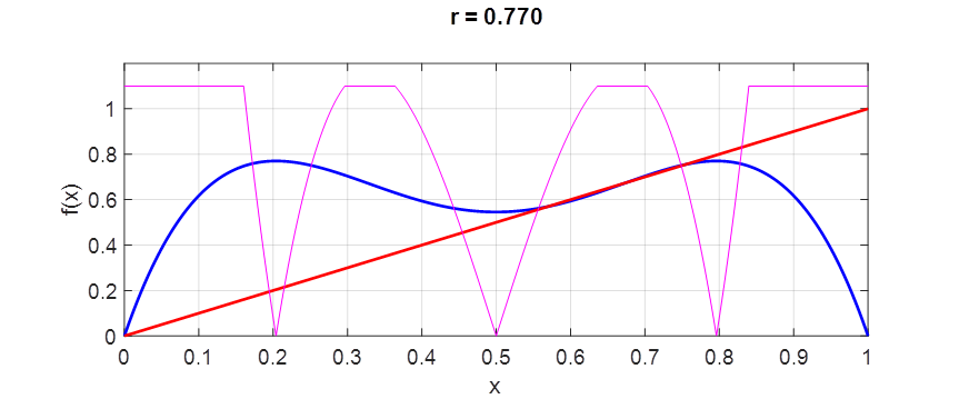
to be period 1. A simple graphical
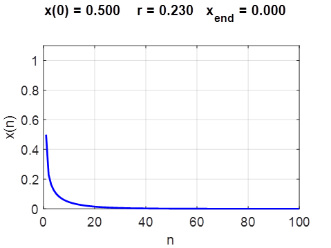
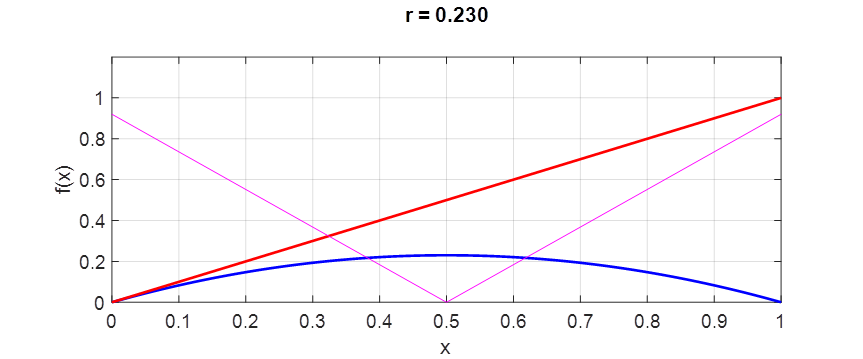
method is shown in figures 5 - 8 for finding the fixed points. The plot shows
the graph of
Fig. 5. Iteration of the map single stable
fixed is chaosLogisticsEq02.m chaosLogisticsEq03.m Whenever the growth parameter is less than 0.25
Fig. 6. Iteration of the map Since The value of the intersection point agrees with the analytical value
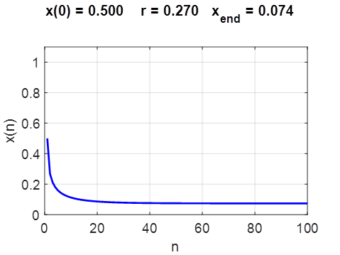
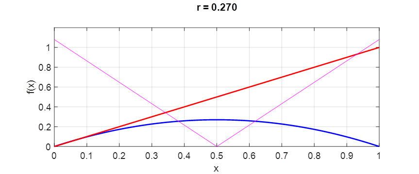
Fig. 7. Iteration of
the [1D] map
line y = x gives the two fixed points,
population The value of the intersection point agrees with the analytical value
When
Fig. 8. Iteration of
the [1D] map
is not a stable fixed point since
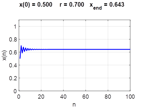
chaosLogisticsEq02.m chaosLogisticsEq03.m
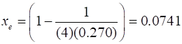
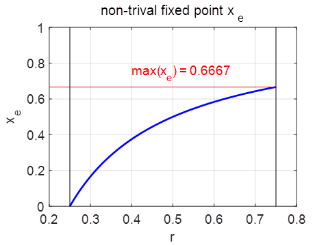
The maximum
value for the stable fixed point is
Fig. 9. The period 1
stable equilibrium point
All trajectories in the neighbourhood of a stable fixed will be attracted to it. chaosLogisticsEq03.m PERIOD DOUBLING
DYNAMICS The
bifurcation diagram shown in figure 10 shows an expanded version of the
figure 1 plot. It clearly shown the change in the dynamics in the evolution
of the population when
Fig. 10. Bifurcation diagram
- plot of the iterated values of of the growth
parameter r
populations to oscillation and period doubling to chaotic behaviour and region of periodic behaviour within the region of chaos. chaosLogisticsEq01.m When
and there are now two attractors of f(x) with fixed points
Fig. 11. Period 2 dynamics chaosLogisticsEq02.m chaosLogisticsEq03.m
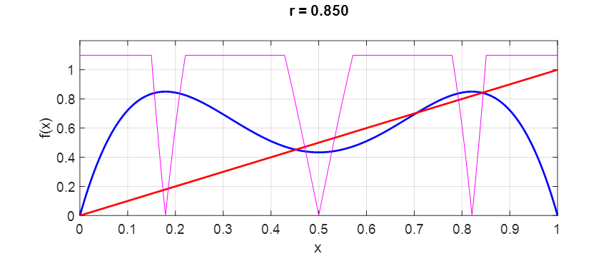
Fig. 12. Period 2 dynamics chaosLogisticsEq02.m chaosLogisticsEq03.m The period 2 dynamics is only exhibited in the range
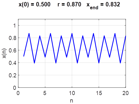
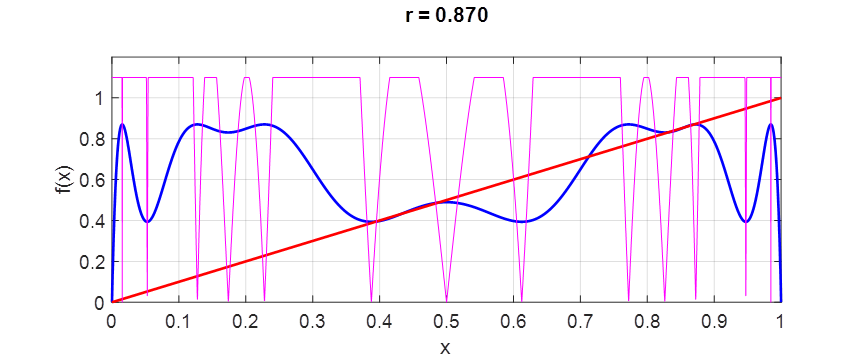
Fig. 13. Period 4 dynamics Increasing r again will lead to further bifurcations. This phenomenon is called period-doubling period 1 à period 2 à period 4 à period 8 à period 16 à . . . Fig. 14. Period 8 dynamics Increasing r again
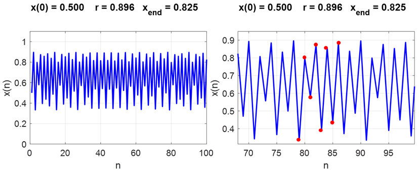
Fig. 15. Population orbits in the chaotic
regime
Fig. 16. Bifurcation diagram. Plot of iterated
values of x(n) as a
function of the growth rate r. chaosLogisticsEq01.m
Fig. 17. Period 1 orbit in a narrow window within the region of chaos. chaosLogisticsEq02.m Figure 18 shows another animated view of the changing population dynamics for increasing values of the growth parameter r.
Fig. 18. The population orbit for increasing values of the growth parameter r. chaosLogisticsEq02.m Period doubling
window In the period doubling
window, periodic motion again occurs where odd period dynamics may occur as
shown in figures 19, 20 and 21.
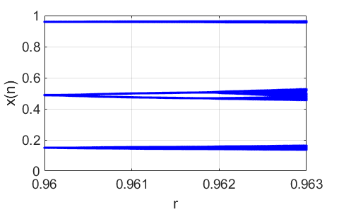
Fig. 20. Bifurcation plot in period doubling
window. chaosLogisticsEq01.m
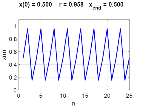
Fig. 21. Period 3
dynamics
Fig. 22. Period 6
dynamics produced by the bifurcation of the period
3 dynamics PERIOD DOUBLING
– FINDING THE FIXED POINTS OF THE DYNAMICS The Script chaosLogisticsEq04.m can be
used to find the fixed points and identify those points which are stable for
any value of the growth parameter r. The input parameters for the Script are the growth factor r A section of the Script chaosLogisticsEq04.m: syms x % Input growth factor r >>>>> r = 0.960; % Input dynamics period P = 1, 2, 3, ... , 8
>>>>> P = 6; % ITERATIONS ========================================================= % [1D] mapping functions f1 = 4*r*x*(1-x); f2 = 4*r*f1*(1-f1); f3 = 4*r*f2*(1-f2); f4 = 4*r*f3*(1-f3); f5 = 4*r*f4*(1-f4); f6 = 4*r*f5*(1-f5); f7 = 4*r*f6*(1-f6); f8 = 4*r*f7*(1-f7); if P == 1; f = f1;
end if P == 2; f = f2;
end if P == 3; f = f3;
end if P == 4; f = f4;
end if P == 5; f = f5;
end if P == 6; f = f6;
end if P == 7; f = f7;
end if P == 8; f = f8;
end % Solve f(xe) = xe eq1 = f - x; % Fixed points xe
= vpasolve(eq1); % Gradient df/dx df
= gradient(f,[x]); % Symbolic to numeric f_dash
= subs(df(1),x,{xe}); % Print results to Command window output(r,
xe, f_dash, P) For the interval 0 < r < ¾, the eventual behaviour
after many iterations is known – the population becomes extinct or is
attracted to an equilibrium (fixed) population
Simulations r = 0.240000 Dynamic period P = 1 xe = -0.041667
f_dash = 1.040 xe = 0.000000
f_dash = 0.960 Stable fixed points xe = 0.000000
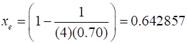
f_dash = 0.960 r = 0.740000 Dynamic period P = 1 xe = 0.000000
f_dash = 2.960 xe =
0.662162 f_dash = -0.960
Stable fixed points xe = 0.662162
f_dash = -0.960 fixed point x1 = 0.662162
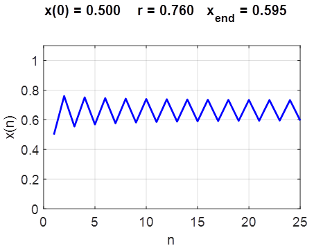
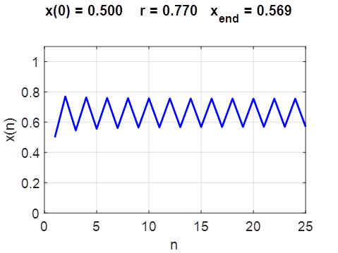
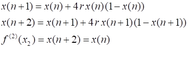
What happens when the value of r is slightly increased slightly above 3/4? We know from our observations the single fixed point becomes unstable and gives birth (bifurcates) to a cycle of period 2. The population x returns to the same value only after every second iteration the range
We can solve this set of equations to find all the fixed points As r is increased
further, eventually the magnitude of the [1D] mapping function Simulations r = 0.760000 Dynamic period P = 1 xe = 0.000000 f_dash = 3.040
xe = 0.671053 f_dash = -1.040 r = 0.760000 Dynamic period P = 2 xe = 0.000000
f_dash = 9.242 xe
= 0.598356 f_dash = 0.838
xe
= 0.671053 f_dash = 1.082
xe
= 0.730591 f_dash = 0.838
Stable fixed points xe = 0.598356
f_dash = 0.838 xe = 0.730591
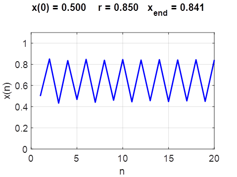
f_dash = 0.838 r = 0.862300 Dynamic period P = 2 xe =
0.000000 f_dash = 11.897
xe
= 0.440028 f_dash = -0.999
xe
= 0.710078 f_dash = 2.100
xe
= 0.849894 f_dash = -0.999
Stable fixed points xe = 0.440028
f_dash = -0.999 xe = 0.849894
f_dash = -0.999 r = 0.862400 Dynamic period P = 4 Stable fixed points xe = 0.437181
f_dash = 0.998 xe = 0.442748
f_dash = 0.998 xe = 0.848787
f_dash = 0.998 xe = 0.851093
f_dash = 0.998 r = 0.886010 Dynamic period P = 4 Stable fixed points xe = 0.363309
f_dash = -0.999 xe = 0.523572
f_dash = -0.999 xe = 0.819792
f_dash = -0.999 xe = 0.884041
f_dash = -0.999 r = 0.886030 Dynamic period P = 8 Stable fixed points xe = 0.362731
f_dash = 0.997 xe = 0.363843
f_dash = 0.997 xe = 0.522372
f_dash = 0.997 xe = 0.524814
f_dash = 0.997 xe = 0.819249
f_dash = 0.997 xe = 0.820326
f_dash = 0.997 xe = 0.883848
f_dash = 0.997 xe = 0.884256
f_dash = 0.997 r = 0.891100 Dynamic period P = 8 Stable fixed points xe = 0.346767
f_dash
= -0.999 xe = 0.374766
f_dash = -0.999 xe = 0.490614
f_dash = -0.999 xe = 0.554267
f_dash = -0.999 xe = 0.807407
f_dash = -0.999 xe = 0.835197
f_dash = -0.999 xe = 0.880603
f_dash = -0.999 xe = 0.890786
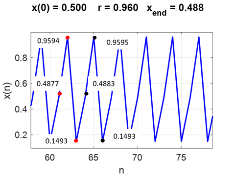
f_dash = -0.999 r = 0.960000 Dynamic period P = 3 xe
= 0.000000 f_dash = 56.623
xe
= 0.149407 f_dash = -0.875
xe
= 0.169434 f_dash = 2.744
xe
= 0.488004 f_dash = -0.875
xe
= 0.540388 f_dash = 2.744
xe
= 0.739583 f_dash = -6.230
xe
= 0.953736 f_dash = 2.744
xe
= 0.959447 f_dash = -0.875
Stable fixed points xe = 0.149407
f_dash = -0.875 xe = 0.488004
f_dash = -0.875 xe = 0.959447
f_dash = -0.875
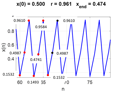
period doubling window in chaotic region r = 0.962000 Dynamic period P = 6 Stable fixed points xe = 0.144093
f_dash = 0.186 xe = 0.153195
f_dash = 0.186 xe = 0.474083
f_dash = 0.186 xe = 0.498668
f_dash = 0.186 xe = 0.958418
f_dash = 0.186 xe = 0.960993
f_dash = 0.186
period doubling window in chaotic region MATLAB Below are segments of the code to investigate the dynamics of the one-dimensional map for the logistic difference equation. chaosLogisticsEq01.m animation x vs n and bifurcation diagram % Initial condition
0 <= x0 <= 1 x0 = 0.25; % Control parameter 0 <= r <= 1 rMin
= 0.10; rMax
= 0.99; Nr = 501; r = linspace(rMin,rMax,Nr); % Number of iterations N = 100; % Logistic Equation x = zeros(N,Nr); xEND
= zeros(Nr,1); for k = 1:Nr
x(1,k) = x0; for c = 1:N-1
x(c+1,k) = 4*r(k)*x(c,k)*(1-x(c,k)); end
xEND(k) = x(c+1,k); end chaosLogisticsEq02.m x vs n % Control parameter 0 <= r <= 1 r = 0.76; % Initial condition
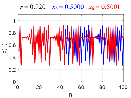
0 <= x0 <= 1 x0 = 0.5001; % Number of iterations N = 25; % Logistic Equation x = zeros(N,1); x(1)
= x0; for c = 1:N-1
x(c+1) = 4*r*x(c)*(1-x(c)); end xEND = x(c+1); xSTABLE = 1-1/(4*r); chaosLogisticsEq03.m [1D] logistic map function f(x) vs x % INPUTS
============================================================== % Period
p = 1, 2, 4, 8 p = 1; % Control parameter 0 <= r <= 1 r = 0.76; % Number of iterations N = 5001; % SETUP
============================================================= % Population x = linspace(0,1,N); dx = x(2) - x(1); % Logistic Difference Equations for period doubling f1 = iterate(x,r); f2 = iterate(f1,r); f3 = iterate(f2,r); f4 = iterate(f3,r); f5 = iterate(f4,r); f6 = iterate(f5,r); f7 = iterate(f6,r); f8 = iterate(f7,r); if p == 1; f = f1;
end if p == 2; f = f2;
end if p == 4; f = f4;
end if p == 8; f = f8;
end % Gradient df/dx gradF
= gradient(f,dx); % FIXED POINTS: Intersection points x and f(x) interSections
= find(abs(f-x) <= 0.001); % xIS = x(interSections); n = 0; xe(1) =
0; for c = 1 : length(interSections) if abs(gradF(interSections(c))) < 1 n
= n+1; xe(n) = x(interSections(c)); end end The logistic difference equation is an exceptionally simple model
of the population growth for butterflies who lay eggs their
eggs in year n and their offspring
are born in year
References http://www.people.vcu.edu/~hsedagha/Sedaghat-CRC_Handbook.pdf H. Gould & J. Tobochnik An Introduction to Computer Simulation Methods (Part 1) R. M. May Simple Mathematical Models with Very Complicated Dynamics, Nature 261, 459 (1979) |