A NUMERICAL APPROACH
TO THE PHYSICS OF THE ENVIRONMENT AND CLIMATE
Ian Cooper
matlabvisualphysics@gmail.com
THE VERTICAL PROFILE OF THE
ATMOSPHERE
MATLAB
Download directory
https://drive.google.com/drive/u/3/folders/1j09aAhfrVYpiMavajrgSvUMc89ksF9Jb
https://github.com/D-Arora/Doing-Physics-With-Matlab/tree/master/mpScripts
Scripts
climate.m
The atmospheric temperature
profile data is stored in the vectors ZD and TD.
Using this data, the
pressure and density profiles are calculated and plotted.
MODEL PARAMETERS:
symbol quantity [value units]
m mass
of a parcel of air [kg]
n number of moles [mol]
N number of molecules [
- ]
M molar mass [kg.mol-1]
MA molar
mass dry air [MA = 0.029 kg.mol-1]
Mw molar
mass water vapour [Mw = 0.018 kg.mol-1]
x,
y, z Cartesian
coordinates [m km]
u,
v, w Cartesian velocity components [m.s-1]
V volume [m3]
dV volume
element [dV = dx dy dz]
![]() density
of air parcel [kg.m-3]
density
of air parcel [kg.m-3]
![]() dry
air density [
dry
air density [![]() = 1.29 kg.m-3 T = 0 oC = 273 K]
= 1.29 kg.m-3 T = 0 oC = 273 K]
[![]() = 1.19 kg.m-3 T = 25 oC = 288 K]
= 1.19 kg.m-3 T = 25 oC = 288 K]
T temperature [K oC]
p pressure [Pa hPa]
![]() change
in internal energy [J]
change
in internal energy [J]
W work [J]
Q heat
exchanged with system [J]
p0 atmospheric
pressure at
Earth’s
surface [p0 = 1013.25 hPa = 1.01325x10⁵ Pa]
g acceleration
due to gravity [m.s-2]
g0 acceleration
due to gravity
at
Earth’s surface [g0 = 9.80665 m.s-2]
R Universal
gas constant [R = 8.314 J.K-1.mol-1]
Rd gas
constant dry air [Rd = 287 J.K-1.kg-1]
kB Boltzmann
constant [kB = 1.38065x10⁻²³ J.K-1]
NA Avogadro’s
number [NA = 6.02214 molecules. mol-1]
cpd constant-pressure
specific heat
for dry air [cpd = 1004.65805 J.kg-1.K-1]
ME mass
of Earth [ME = 5.9722x1024
kg]
RE radius
of Earth [RE = 6.3743x10⁶ m]
G
Gravitation constant [G = 6.67408 x10⁻¹¹ N.m2.kg-2]
THE ATMOSPHERE
The
atmosphere contains a few highly concentrated gases, such as nitrogen (78%),
oxygen (21%), and argon (0.93%), carbon dioxide (0.035%) and many trace gases,
such as methane, ozone and nitrous oxide. To a good approximation the gases of
the atmosphere can be assumed to obey the laws for an ideal gas.
The
most characteristic feature of the atmosphere is its vertical temperature
distribution profile. From the ground up to a mean altitude of 11 km (8 km at
the poles and 17 km at the equator) lies the troposphere. Nearly all
meteorological phenomena occur within this layer (wind, cloud formation and
precipitation). Above the troposphere is the stratosphere (~11 km to ~ 50 km)
where airflow is primarily horizontal. The narrow layer separating the
troposphere and stratosphere is called the tropopause. Beyond the stratosphere is are the
layers stratopause
(~ 50 km), mesosphere
(~50 km to ~90 km), mesopause (~90 km) and the thermosphere
(> ~90 km).
The
temperature profile of the atmosphere is shown in figure 1. The figure is
generated using the Matlab script climateG.m using the temperature data from Fundamentals of Atmospheric Modelling by
Mark Z. Jacobson
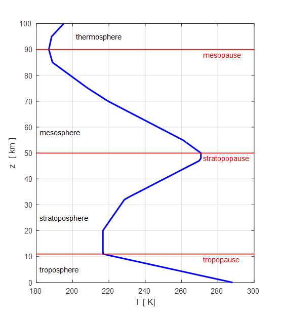
Fig. 1. Vertical temperature profile of
the atmosphere. (Script climateG.m)
Other
important characteristics of air are its pressure and density. These parameters
vary with altitude, latitude, longitude, and season. Using the equation for an
ideal gas, it is possible to calculate the vertical profiles of the pressure
and density numerically from the temperature profile.
Consider
a parcel of air in static equilibrium as shown in figure 2. The forces acting
upon the parcel are the gravitational force FG
and the pressure gradient force FP such
that the net force is zero ![]() . The pressure gradient force at any
altitude is due to the weight of the entire column of air vertically above it.
. The pressure gradient force at any
altitude is due to the weight of the entire column of air vertically above it.
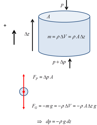
Fig. 2. Forces acting on a parcel of air.
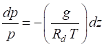
Hence,
the vertical pressure gradient is
(1) 
and the horizontal pressure at
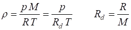
any altitude is a constant. Equation (1) is known the hydrostatic equation. Since the
density ![]() is a function of
altitude, we need to express the density as a function of temperature T.
is a function of
altitude, we need to express the density as a function of temperature T.
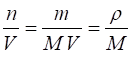
The
equation of
state for an ideal gas describes the relationship among pressure,
volume, and absolute temperature.
(2) ![]()
(3) 
Combining equations (1) and
(3), we obtain
(4) 
Equation (4) can be solved to
find the variation in pressure and density as functions of altitude. However,
equation (4) is difficult to solve since the temperature T is also a function of altitude z. Often many
approximations are used to find a solution to equation (4) such as assuming T = constant. Equation (4) can be solved using
numerical methods to directly integrate the equation from the Earth’s
surface (p = p0, z = 0) to
an altitude z.
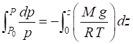
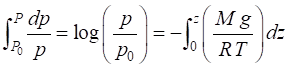
(5) 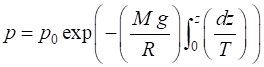
Once the variation of pressure
with altitude is known, then the variation in density is given by
(3)
To evaluate equation (5), the
published data* for the variation in temperature T with altitude z is used. Part of the
Script climateG.m to evaluate
equation (5) is
num = length(zD);
PD = zeros(num,1);
PD(1) = p0;
for c = 1:num-1
PD(c+1) = PD(c) * exp((-2*gD(c)./R_d)*(zD(c+1)-zD(c)) / (TD(c+1) + TD(c)));
end
rhoD = PD./(R_d.*TD');
zD and
TD are the vectors for the published data*.
* Fundamentals of
Atmospheric Modelling
by Mark Z. Jacobson
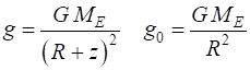
The
acceleration due to gravity g is also
a function of altitude z and is
calculated from Newton’s Law of Gravitation
(6) 
The change in g with z is insignificant since z
<< RE.
Figures 3 and 4 show the
variation in the acceleration due to gravity, atmospheric temperature,
atmospheric pressure and density as functions of altitude.
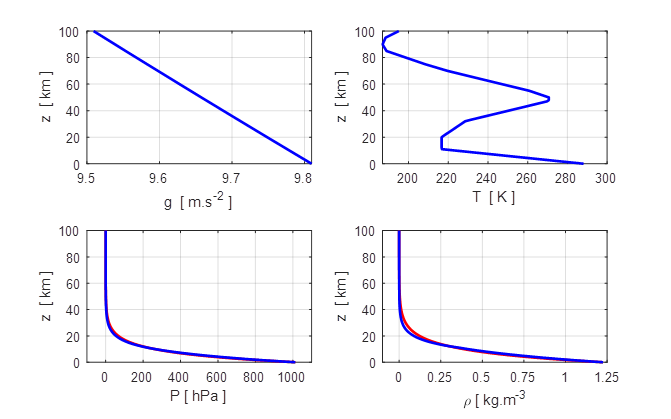
Fig.
3. Variation of the
acceleration due to gravity g,
temperature T, pressure P and density ![]() with altitude z. The
red curves in the pressure and density show that
there is an excellent fit for exponential decreases in both the pressure and
density with altitude.
with altitude z. The
red curves in the pressure and density show that
there is an excellent fit for exponential decreases in both the pressure and
density with altitude.
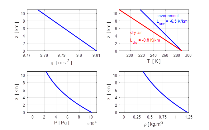
Fig. 4.
Variation of the acceleration due to gravity g, temperature T,
pressure P and density ![]() with altitude z in
the troposphere.
with altitude z in
the troposphere.
The pressure diagram shows air
in the atmosphere is concentrated in a thin shell above the Earth’s surface.
99.7%
atmosphere below 40 km
95% atmosphere below 20 km
74% atmosphere
below 10 km
47%
atmosphere below 5 km
In
figure (3) exponential decay curves (red) were
added to the plots for the pressure and density. The Matlab Curve Fitting Tool was
used to find the exponential equations for the fits
![]()
where H is known as the scale height.
Pressure
![]()
Density
![]()
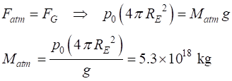
We can now easily estimate the
mass Matm
of the atmosphere
At the Earth’s surface
In the troposphere the
temperature falls linearly with increasing altitude
![]()
where
![]() is the surface
temperature and
is the surface
temperature and ![]() is the vertical
thermal lapse rate.
is the vertical
thermal lapse rate.
The values for the T0 and Lenv (environmental
lapse rate) as shown in figure 4 are calculated using the Matlab function fitlm
F = find(zD>1e4,1);
F = 1:F;
LR = fitlm(zD(F),TD(F))
Lcoeff = LR.Coefficients.Estimate
Lintercept = Lcoeff(1)
Lslope = Lcoeff(2)*1e3
The
results are: T0 = 288 K and Lenv =
- 6.49 K.km-1
We
can calculate the dry air lapse rate using the first law of
thermodynamics and the ideal gas
equations. The first law of thermodynamics states that when heat Q is exchanged with an isolated system,
the system does work W and the
internal energy of the system changes ![]() (when there is a change in the internal energy of the system,
its temperature changes).
(when there is a change in the internal energy of the system,
its temperature changes).
![]()
Consider a parcel of air that
is displaced upward without any exchange of heat with the surrounding air Q = 0. This process when Q = 0 is called adiabatic. Since the pressure
decreases with height, the parcel of air will expand and do work on its
surroundings which results in a fall in its temperature and decrease in its
internal energy.
For an adiabatic
process
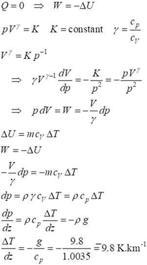
The
adiabatic dry air lapse rate within the troposphere is -9.8 K.km-1.
The adiabatic dry air lapse rate has a larger magnitude than the environmental
lapse rate -6.5 K.km-1. With humid air the lapse rate varies between
– 5 to -10 K.km-1.