|
CHAOTIC DYNAMICAL SYSTEMS A
DRIVEN DAMPED PENDULUM Ian Cooper matlabvisualphysics@gmail.com DOWNLOAD DIRECTORIES
FOR PYTHON CODE cs_006_01.py Solves the differential equation that governs the dynamics of a simple
damped and driven pendulum. The nonlinear ODE for the pendulum system is
extremely sensitive to the model’s parameters and initial conditions. All
input parameters much be chosen with care. Values mostly used in the
simulations are those used by J.R. Taylor in his excellent book Classical
Physics. cs_006_02.py Lyapunov exponent cs_006_03.py Bifurcation diagram cs_006_04.py Poincare section plot: for different values of the
drive strength CHAOTIC
DYNAMICAL SYSTEMS Chaotic
phenomena appear in many real-life situations from meteorology, medicine, biological
systems, ecological systems, fluid dynamics, economics, and many other
fields. This article will consider a sinusoidally driven and damped simple
pendulum (DDP) as a dynamical system that exhibits chaotic motion. It is
important to realize that chaotic behaviour and random behaviour are not the
same. Chaotic systems are deterministic, you can predict the time evolution
of the system for a given set of initial conditions. However, even for
extremely small changes in the initial conditions for chaotic systems, the
time evolution will result in very different trajectories, there being no
element of randomness in the trajectory. Chaotic dynamical systems are
therefore unpredictable but are not random in nature as any difference in the
initial conditions are amplified as the system evolves with time to give
enormously different results. DEFINITIONS Dynamical system: A
system whose behaviour expressed in terms of position, velocity and
acceleration may be modelled by a set of differential equations together with
a set of initial conditions. Non-linear dynamical system:
A system is non-linear if the set of
differential equations contain non-linear terms like, x2, xy, ex, sin(x), etc. Deterministic system: The
solution of the differential equations is unique (one and only one solution)
for a given set of initial conditions for deterministic systems. State: Is
a set of specifications of the motion at any time t0 that
is complete enough to determine uniquely the motion of the system at all time
t > t0 Phase space: Phase
space is the space of all possible states of a dynamical system. Fixed point: A
dynamical system is in equilibrium at a fixed point where each state variable
has a fixed constant value. Fixed points may be classified as stable,
unstable or semi-stable. Orbit (trajectory): The set
of points in phase space that satisfy the differential equations that govern
the system. For a fixed point, the orbit is a single point. Periodic orbit: The set of points in the solution of the differential equations repeat themselves and the motion is said to be periodic. Limit cycle: A
closed curve in phase space towards which an orbit may evolve as Attractor: The set of points in space towards which the dynamical system evolves as t gets larger. This may be towards a single fixed-point or a limit cycle or an extremely complicated set of points. Chaotic attractor: If two sets of initial conditions that are almost identical, results in the two orbits diverging exponentially, then the attractor is said to be chaotic. Only non-linear dynamical systems have chaotic attractors. Small differences in the initial conditions lead to widely divergent orbits in phase space making them in practice unpredictable although they are deterministic. Poincare section: A
Poincare map is the intersection of a periodic orbit in the phase (state)
space of a continuous dynamical system with a certain lower-dimensional
subspace, called the Poincare section. The Poincare section preserves many
properties of periodic and quasiperiodic orbits of the original system and
has a lower-dimensional state space. So, it is often used for analysing the
original system in a simpler way. A Poincare map differs from a recurrence
plot in that space, not time, determines when to plot a point. Bifurcation diagram: A bifurcation
is a period-doubling, a change from an N-point attractor to a 2N-point
attractor, which occurs when a control parameter r is changed. A
Bifurcation diagram is a visual summary of the succession of period-doubling
produced as r increases. Bifurcation diagrams are analysed by varying
one parameter at a time and keeping others fixed. SIMPLE
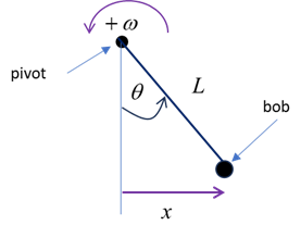
PENDULUM (free, damped, driven motion) We first
consider a simple rigid pendulum (zero mass) of length L that is
constrained to move along an arc of a circle centred at a pivot point. The
angular displacement w.r.t. the vertical is θ, the
angular velocity is
The
equation of motion for the pendulum with damping and subjected to a
sinusoidal driving force applied at the pivot is (1) where t time [s]
g acceleration due to gravity [g = 9.80 m.s-2] L length of pendulum [m] To solve equation 1 using
the Python function odeint, we need
to write this second-order differential equation as the system of two
first-order equations (2) For small amplitude
free vibrations of the simple pendulum, its natural period T0,
frequency f0 of vibration, and angular frequency are (3) The pivot point is
taken as the origin (0,0) and in Cartesian coordinates, to the right is the
+X direction and up is the +Y direction. The position of the bob at the end
of the pendulum is: Horizontal
displacement at any time t is (4)
Vertical position at
the end of the pendulum is (5)
The two fixed-point of
the system occur when Any small changes in
the damping, driving force strength, or driving force frequency may result in
very different trajectories of the pendulum. It is not possible for the
motion of the pendulum to be chaotic if the forces acting of the pendulum are
only the gravitational force and the damping force. Chaos can only occur if an external driving force also acts on
the system and the driving frequency is less than the natural frequency of
oscillation If SIMULATIONS Free
motion of the pendulum with a small initial displacement cs_006_01.py An
undamped pendulum with zero driving force acting will vibrate with
approximately simple harmonic motion (SHM) when it
is given a small disturbance from its equilibrium position. Python Console Initial conditions
theta(0)/pi = 0.100 omega(0) = 0.0000 rad/s Damping: b = 0.000 Free vibration T0 = 0.667 s f0 = 1.500 Hz w0 = 9.425 rad/s Driving force
gamma = 0.000 TD = 1.000
s fD =
1.000 Hz wD
= 6.283 rad/s Results Peaks t vs x: Tpeak = 0.671
s fPeaks =
1.491 Hz psd:
TPeak = 0.664 s fPeak = 1.505 Hz PLOTS Time evolution plots
Phase space plots The [2D] plot of
Frequency spectrum The power spectral density psd is plotted against frequency f. The red
vertical line shows the natural frequency fo
and the magenta line for the driving
frequency fD .
The pendulum oscillates at
its natural frequency (1.5 Hz) and its motion is described as simple harmonic
motion (SHM). The Fourier Transform is calculated
by direction integration of the Fourier Transform integral. For small amplitude oscillation the
pendulum corresponds to a linear system. Free
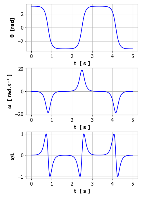
motion of the pendulum with a large initial displacement cs_006_01.py The pendulum is released
very close to its vertical position (unstable fix-point) Python Console Initial conditions
theta(0) = 3.138 rad omega(0) = 0.0000 rad/s Damping: b = 0.000 Free vibration T0 = 0.667 s f0 = 1.500 Hz w = 9.425 rad/s Driving force
gamma = 0.000 TD = 1.000
s fD =
1.000 Hz wD
= 6.283 rad/s Results Peaks t vs x: Tpeak = 1.112
s fPeaks =
0.899 Hz psd:
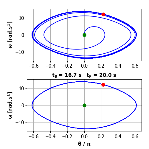
TPeak = 1.087 s fPeak = 0.920 Hz Plots Time evolution plots
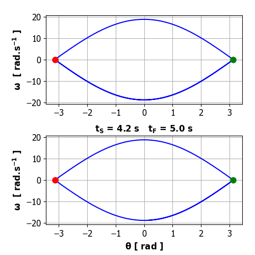
Phase space plots Green dot gives initial state and red dot final state. Lower graph shows the orbit
only for the time interval from tS
to tF. so that any initial
transient vibrations are removed.
Frequency spectrum The power spectral density psd is plotted against frequency f. The red
vertical line shows the natural frequency fo
and the magenta line for the driving
frequency fD (not
shown as driving strength is zero). Notice the two predominant peaks in the
frequency spectrum at 0.90 Hz and 1.50 Hz (natural frequency) and a small
peak at 0.31 Hz.
The motion is anything
but SHM with a very large initial angular
displacement. The period of motion is longer than the natural period or the
frequency of vibration is lower than the natural frequency It is easy to show if
a fixed-point is stable or unstable by considering a small increment away
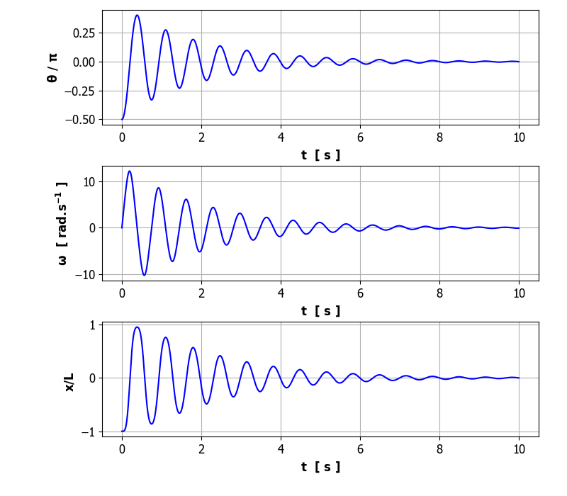
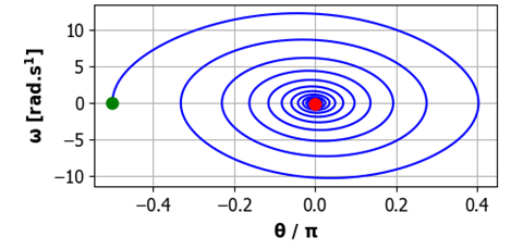
from the equilibrium point, for example, Free
motion of the pendulum with a damping
Many aspects of damped
vibrational motion such overdamped, underdamped, and critical damping can be
explored using the code cs_006_01.py. Python
Console Model
Parameters theta(0)/pi =
-0.500 omega(0) = 0.0000 rad/s Damping: b = 0.500 Driving
force gamma = 0.000 TD = 1.000 s fD = 1.000
Hz wD =
6.283 rad/s Time
span time steps = 5999 tMax = 10.000 s Free
vibration T0 = 0.667 s f0 = 1.500 Hz w0 = 9.425 rad/s Results Peaks
t vs x: Tpeak
= 0.675 s fPeaks
= 1.482 Hz psd: TPeak =
0.632 s fPeak
= 1.581 Hz Plots Time evolution
Phase space plot
Frequency spectrum
The motion is attracted to the fixed-point
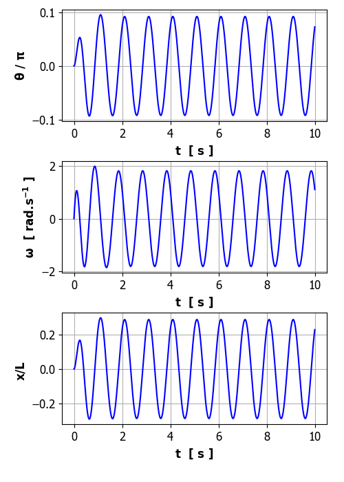
(steady-steady or equilibrium position) of the system Forced
motions of the pendulum with damping The system is excited by
some external sinusoidal driving stimulus with amplitude The default parameters are
mainly used for each simulation and only the drive strength Relatively weak driving strength
Python Console Model Parameters
theta(0)/pi = 0.000 omega(0) = 0.0000 rad/s Damping: b = 3.000 Driving force
gamma = 0.200 TD = 1.000
s fD = 1.000
Hz wD =
6.283 rad/s Time span
time steps = 5999 tMax = 10.000 s Free vibration T0 = 0.667 s f0 = 1.500 Hz w0 = 9.425 rad/s Results Peaks t vs x: Tpeak = 0.985
s fPeaks =
1.015 Hz psd:
TPeak = 0.945 s fPeak = 1.059 Hz Plots Time evolution The pendulum motion is to a
good approximation SHM.
Phase space After the initial transient
motion, the motion of the pendulum becomes periodic.
Frequency spectrum The system vibrates at the driving frequency (fD
= 1.00 Hz) and not the natural frequency
of vibration (f0 = 1.50 Hz).
We see that the driver and
the response have the same period. Something which intuition from linear problems
would say is obvious. The response has two regimes: (1) the decay of an
initial transient motion and (2) the steady oscillations at the frequency of
the driving signal. The amplitude of the response depends upon the energy
balance between the energy supplied by the external driving force and the
energy dissipated by the system due to the damping. The phase space plot
exhibits a regular orbit which is independent of the initial conditions
except for the initial transients which does depend upon the initial
conditions. The motion approaches a unique attractor in which the pendulum
oscillates sinusoidally with exactly the same frequency as the driving force.
In conclusion for the motion
of the linear DDP with a sinusoidal driving force: (1) There is a unique attractor which the motion approaches,
irrespective of the initial conditions applied. (2) The motion of the attractor is itself sinusoidal with frequency
exactly matching the drive frequency. Weak driving strength Python Console Model Parameters
theta(0)/pi = 0.000 omega(0) = 0.0000 rad/s Damping: b = 3.000 Driving force
gamma = 0.900 TD = 1.000
s fD =
1.000 Hz wD
= 6.283 rad/s Time span
time steps = 5999 tMax = 20.000 s Free vibration T0 = 0.667 s f0 = 1.500 Hz w0 = 9.425 rad/s Results Peaks t vs x: Tpeak = 0.341
s fPeaks =
2.930 Hz psd:
TPeak = 0.978 s fPeak = 1.023 Hz Plots Time evolution After
4 cycles (4 s) the motion settles down to a regular oscillation that looks
like sinusoidal with a period equal to the driving frequency. However, the
regular oscillations are not sinusoidal since the curve is flatter at the
extremes.
Phase space The motion of the pendulum
is periodic with a period equal to the driving frequency (fD
= 1.00 Hz),
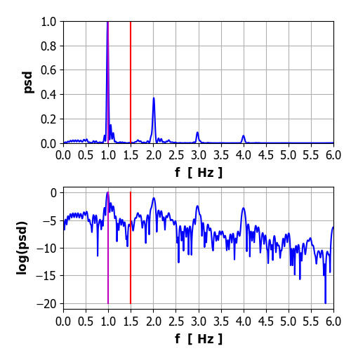
Frequency spectrum Most of the energy supplied
by the driving force to the pendulum system excites the fundamental frequency
(driving frequency fD = 1.00 Hz).
However, small amount of energy also excites the 3rd harmonic (3.00 Hz) and
the 5th harmonic (5.00 Hz) due to the non-linearity of the DDP
system. For the nth harmonic, the period is given by
So, there is strong evidence
(not a proof) that a periodic attractor is approach with a period exactly
equal to the driving force. The boundary between weak
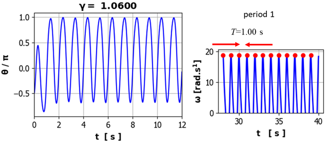
and strong driving stimulus is around Strong driving strength Python Console Initial conditions
theta(0)/pi = 0.000 omega(0) = 0.0000 rad/s Damping: b = 2.356 Free vibration T0 = 0.667 s f0 = 1.500 Hz w0 = 9.425 rad/s Driving force gamma = 1.060 TD = 1.000 s fD = 1.000
Hz wD =
6.283 rad/s Results Peaks t vs x: Tpeak = 0.384
s fPeaks =
2.607 Hz psd:
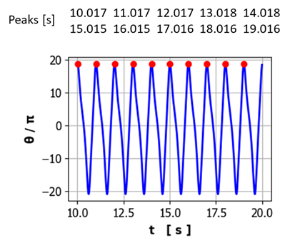
TPeak = 1.009 s fPeak = 0.991 Hz Plots Time evolution Initially there are dramatic
oscillations where the pendulum swings through more than two anticlockwise
rotations then swings back to about
Phase space The phase space plot shows a
single closed orbit after the initial transient period indicating periodic
motion of the pendulum centred around
Frequency spectrum The frequency spectrum is
characterized by the large peak at the driving frequency (f = 1.00
Hz). The motion of the pendulum becomes complicated because of a number of
harmonic oscillations are picked up.
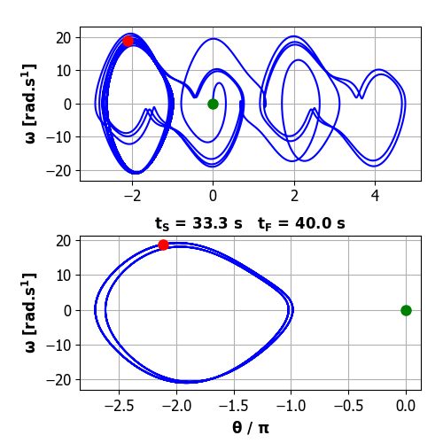
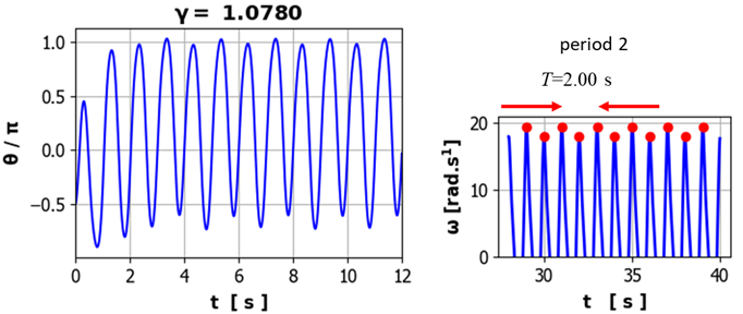
Strong driving strength Period 2 Python Console Initial conditions
theta(0)/pi = 0.000 omega(0) = 0.0000 rad/s Damping: b = 2.356 Free vibration T0 = 0.667 s f0 = 1.500 Hz w0 = 9.425 rad/s Driving force
gamma = 1.073 TD =
1.000 s fD
= 1.000 Hz wD
= 6.283 rad/s Results Peaks t vs x: Tpeak = 0.408
s fPeaks =
2.452 Hz psd:
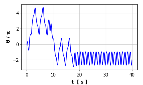
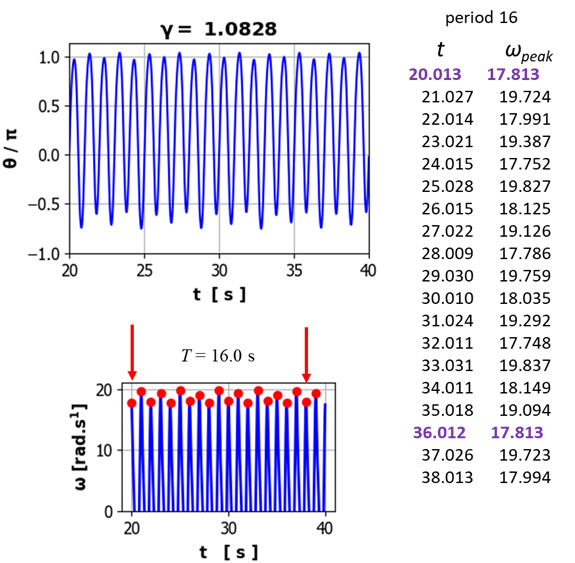
TPeak = 1.007 s fPeak = 0.993 Hz Plots Time evolution There are wild fluctuations
in the position of the pendulum during the first 20 s before a regular
periodic motion is established. On careful examination of the periodic
motion, one will observe that the heights and troughs are not all of the same
height, but vary between two distinct heights and this pattern continues
indefinitely. So, the strong driving force acting on the system results in a
doubling in the period of the pendulum to produce period
2 motion.
Phase space After the initial wild
motion, the phase space plot evolves to two distinct orbits indicating period 2 motion. This behaviour means that
the motion no longer repeats itself every drive cycle but every two drive
cycles, so the period of the pendulum is twice the drive period. We now have
a periodic attractor with period 2.0 s. This phenomenon is known as period doubling
Frequency spectrum
(horizontal displacement for periodic motion) The spectrum is
characterized by the two major peaks at frequencies of 1.0 Hz and 2.0 Hz (fD = 1.00 Hz). Also, some energy is transferred to the higher harmonics.
The motion of the pendulum
is sensitive to small changes in the strength of the driving force. For example,
if we increment the drive strength from 1.073 to 1.075 the attractor shifts
from an orbit around -2
Although the attractor has
period 2, the dominant behaviour is still clearly period 1. Strong driving strength Period 3 There is now an attractor for which a subharmonic
term is dominant and the motion settles down to an attractor that repeats
itself every 3 drive cycles and hence period 3
(T = 3.0 s). Initial conditions theta(0)/pi = 0.000
omega(0) = 0.0000 rad/s
Damping: b = 2.356 Free vibration
T0 = 0.667 s f0 = 1.500
Hz w0 = 9.425 rad/s Driving force gamma = 1.077 TD = 1.000 s fD = 1.000
Hz wD =
6.283 rad/s Results Peaks t vs x:
Tpeak = 0.590 s fPeaks = 1.695
Hz psd: TPeak = 0.984 s fPeak = 1.017 Hz Time evolution The motion quickly
settles down to period 3 motion (T = 3.00 s)
Phase space A single orbit is
established after the initial transient motion.
Frequency spectrum (angular
velocity The subharmonic term becomes
the dominant term in the frequency spectrum .
Initial conditions For a linear oscillator, with
a given set of parameters there is a unique attractor that is independent of
the initial conditions, the eventual motion will be the same once the
transients have decayed away. This is
not the case for a non-linear system as shown below. The initial condition
for the blue curve is
For
the motion with the initial condition Period doubling cascade Simulation parameters: As the driving stength
It is remarkble that the phenomenum of period-doubling is
observed in many non-linear physical systems as a control parameters is incremented.
In all such systems, the period-doubling cascade occurs in the same way, a
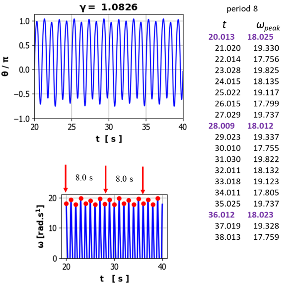
circumstance known as universality. The Feigenbaum Number and Universality The period doubling occurs more and more frequently as
1 à 2
2 à 4 4
à 8 8
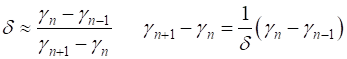
à 16 We can define the Feigenbaum number as For
many non-linear systems, the Feigenbaum number is universal and, in the
limit, as In
our example of the DDP system If
we continue this sequence of period doubling, we will reach a limit, to give
a critical value for For
CHAOTIC
MOTION For
drive strengths greater than about a critical value of The case for
CHAOS
and sensitivity to initial conditions The
other defining feature of chaos is that a trajectory is extremely sensitive
to the initial conditions. For our DDP system with Lyapunov Exponents cs_006_02.py Consider two identical pendulum which are released with
different initial conditions for the angular displacement where the parameter Consider two motions of the pendulum with a small driving
force It is clear from log scale plot, the maxima in the log
scale for
With a moderate drive strength Initial condtions:
Two identical DDPs with a strong driving force
For about 12 s, the motion of both pendulums is erratic
but follow similar orbits and then the orbits diverge exponentially then
levels out.
The above results for pendulums which start with nearly identical
initial conditions indicate that for small or medium forcing, the motions
will converge exponentially whereas for high forcing, the trajectories
diverge exponentially. The pendulum system while obeying deterministic laws
may still exhibit irregular and unpredictable behaviour due to an extreme
sensitivity to initial conditions.
BIRFURCATION DIAGRAM cs_006_03.py The purpose of a bifurcation diagram is to show in a single
plot, the changing periods, alternating periodicity, and chaos as the drive
strength The required steps in plotting a bifurcation diagram are: 1. Choose a large number of evenly spaced values for 2. Choose the initial conditions 3. Solve the equation of motion for DDP for each value of 4. Check for periodicity or non-periodicity when all the
transience has disappeared by examining 5. Plot these values of The bifurcation diagram is very dependent upon choice of
parameters and initial conditions. The following diagrams show the period
doubling cascade effect for initial conditions Bifurcation:
PHASE SPACE ORBITS: POINCARE SECTION cs_006_01.py cs_006_04py A
Poincare section is another way to visualise the motion of chaotic systems.
The Poincare section is a simplified view of a phase space orbit. The phase
space or state-space is the plot of cs_006_01.py Initial
conditions theta(0)/pi =
-0.500 omega(0) = 0.0000 rad/s Damping: b = 2.356 Free
vibration T0 = 0.667 s f0 = 1.500 Hz w0 = 9.425 rad/s Driving
force gamma = 0.600 TD = 1.000 s fD = 1.000
Hz wD =
6.283 rad/s The
orbit spirals inwards in a clockwise direction and rapidly approaches the
period 1 attractor and then continually cycles around the attractor. If the initial angular
displacement is
So, for large t values,
the two orbits become identical and one can not distinguish between the two
different initial conditions. The phase-space plot gives a clearer picture of
the approach to the attractor than the time evolution plots. cs_006_01.py Initial conditions theta(0)/pi =
-0.500 omega(0) = 0.0000 rad/s Damping: b = 2.356 Free vibration T0 = 0.667 s f0 = 1.500 Hz w0 = 9.425 rad/s Driving force gamma =
1.078
TD = 1.000 s fD = 1.000 Hz wD = 6.283 rad/s After the transient motion
has decayed way, the orbit is composed of two distinct loops, and the
attractor is period 2.
cs_006_01.py Initial conditions theta(0)/pi =
-0.500 omega(0) = 0.0000 rad/s Damping: b = 2.356 Free vibration T0 = 0.667 s f0 = 1.500 Hz w0 = 9.425 rad/s Driving force gamma =
1.081
TD = 1.000 s fD = 1.000 Hz wD = 6.283 rad/s After the transient motion
has decayed way, the orbit is composed of four distinct loops, and the
attractor is period 4.
cs_006_01.py CHAOS Initial conditions theta(0)/pi =
-0.500 omega(0) = 0.0000 rad/s Damping: b = 2.356 Free vibration T0 = 0.667 s f0 = 1.500 Hz w0 = 9.425 rad/s Driving force gamma =
1.105
TD = 1.000 s fD = 1.000 Hz wD = 6.283 rad/s There is no closed
orbit, the motion never repeats itself, so the motion is chaotic.
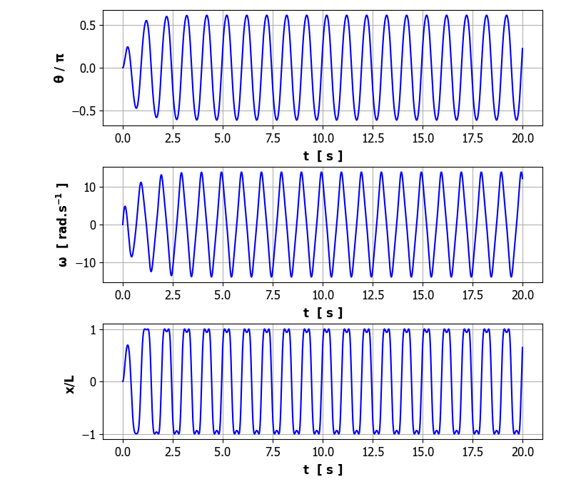
cs_006_01.py ROLLING MOTION Initial conditions theta(0)/pi =
-0.500 omega(0) = 0.0000 rad/s Damping: b = 2.356 Free vibration T0 = 0.667 s f0 = 1.500 Hz w0 = 9.425 rad/s Driving force gamma = 1.400 TD = 1.000 s fD = 1.000 Hz wD = 6.283 rad/s For
large values of the drive strength, we can a rolling motion where the
pendulum swings through a complete revolution each drive cycle. After the
initial transient motion, the motion of the pendulum is perfectly periodic as
the motion in each loop is identical.
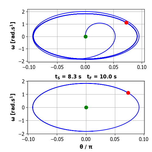
POINCARE SECTION cs_006_04.py There is a way to study chaotic motion that is better than simply plotting the trajectory in phase space because after many cycles it contains too much information to be useful. Consider the phase space plot where points are not plotted at every time step but only at times given by Such a phase space plot is called a Poincare section. If the pendulum oscillates at the driving frequency, then only one point will appear in the Poincare section. If the oscillation has twice the frequency of the driving force, then the Poincare section will have two points. If the motion is not periodic and chaotic the Poincare section will consist of a pattern of points called the attractor. The attractor has a structure that is frequently beautiful even though the motion is unpredictable and chaotic, yet at the same time preserve a coherent global structure. So, in the Poincare section plot, the orbit is not drawn but only points at one drive cycle interval. For periodic motion the Poincare section is not useful, but it is very useful for visualisation of chaotic motion. Period 1
oscillations
For The phase space
plot (red: orbit after transient motion
decayed away) and Poincare section for
Period 2
oscillations For The red trajectory shows the orbit after the
transient motion has decayed away. The motion is period 2 since there are two
loops that make up one period of the oscillation and two dots are show on the
Poincare section.
Poincare
section for chaotic motion Initial conditions theta(0)/pi =
-0.500 omega(0) = 0.0000 rad/s Damping: b
= 1.178 Free vibration T0 = 0.667 s f0 = 1.500 Hz w0 = 9.425 rad/s Driving force gamma = 1.500 TD = 1.000 s fD = 1.000 Hz wD = 6.283 rad/s The pendulum undergoes an erratic rolling motion making many complete revolutions in one direction and then in the other direction, but never repeating itself. The phase space plot is not useful because of the entanglement of the orbit as the pendulum swings through complete revolutions in one direction, then the other.
The
Poincare section and enlargements The
Poincare section contains a subset of all the points of the phase space orbit,
and it is impossible to know what this subset of points will look like, but
we are able to compute and display it. The Poincare section often gives a
very elegant picture by plotting this subset of points which are one drive
cycle apart. The Poincare section is simply not a figure but a fractal where one finds further structure by
enlarging sections of the Poincare section. For example, zooming in a “tongue” is
actually made up of many tongues. If you had plotted enough points, you could
keep zooming in a finding a repetition of the tongue structure. The Poincare
section took about 2 hours to compute and plot. This self-similarity is
one of the features of a fractal. for a chaotic system which can be visualised
as a fractal, the long-term motion is said to be a strange attractor.
|