|
RUNGA-KUTTA FOURTH-ORDER METHOD Numerical Solution
of Ordinary Differential Equations Initial Value
Problems Ian Cooper Any
comments, suggestions or corrections, please email me at |
|
MATLAB DOWNLOAD
DIRECTORY FOR SCRIPTS da_RK01.m Solutions of ODE of
the form da_RK02.m Solutions of ODE of
the form da_RK03.m Sets of First-Order ODEs da_RK04.m Second-Order ODEs
Damped harmonic
oscillator |
|
RUNGE-KUTTA METHOD The purpose of the Runge-Kutta
method is to obtain an approximate numerical solution of an ordinary
differential equation given a set of initial conditions. The Euler method is
in general not recommended for solving ordinary differential equations (ODEs) because it is not very accurate compared to other
methods run at the same step size and is not always stable. The fourth-order Runge-Kutta method described below is adequate for most
practical applications. Problems involving ODEs
can always be reduced to the study of sets of first-order differential
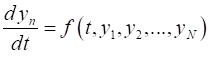
equations. The generic problem in ODEs is thus
reduced to the study of a set of N coupled first-order differential equation for the functions yn, n = 1, 2, 3, … , N having the form
(1) where the functions on the right-hand
side are known. The goal is to find the unknown yn values. The solutions of equation
1 depend upon the boundary conditions applied (known values of the function yn). Only initial value problems where all the yn values are
given at some starting value ts are considered. The fourth-order Runge-Kutta
method is based upon solving a system of equations at each time t with time step h (h = constant is only considered. You can include an
adaptive step size algorithm is greater accuracy is required.
(2A)
(2B)
(2C)
(2D)
(2E)
(2F)
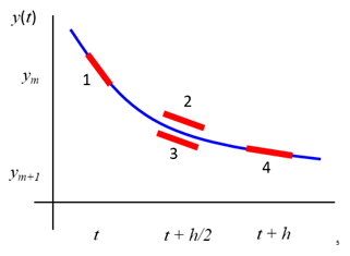
(2G) In each time step the derivative is evaluated
four times: once at an initial point and once at the end point and twice at
the mid-point.
The Runge-Kutta is
not the best and most accurate ODE integrator, but is OK for most
applications and is very easy to incorporate into a Script. An advantage of
the method is that it is self-starting – requires only a value of the
function at a single previous point to obtain functional values ahead. Also,
it is easy to change the step size h at any step in the computation. |
|
Example 1
Exact solution
You can vary the
step size h to find out the largest value of h that still gives an accurate
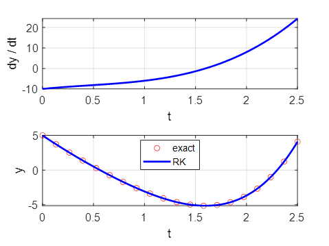
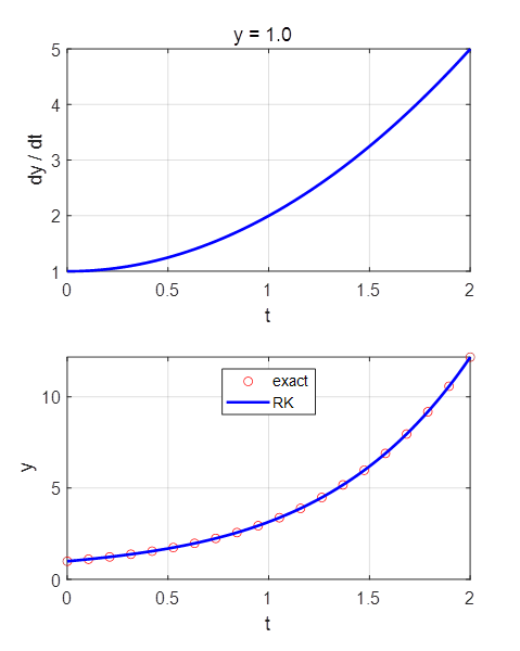
result. Example 2
Exact solution
The ODE is given as a
Matlab function. The function can easy be changed. function f = YDOT(t,y) % f = t + y;
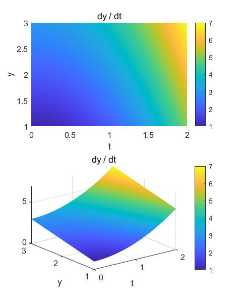
f = t.^2 + y; end The input parameters
are given in the Input section of the Script %
>>>>> Number of
grid points N = 200; %
>>>>> t variable tMin = 0; tMax = 2; %
>>>>> initial
value for y variable y = zeros(1,N); y(1) = 1; The ODE is solved in
the Setup section of the Script % SETUP
============================================================== % t interval and
step size t = linspace(tMin,tMax,N); h = t(2) - t(1); % yDot variable as a function of t at y(nY)
(calls function YDOT) nY = 1; yDot = YDOT(t,y(nY)); % Compute y and yDdot values as a function of time ===================== for n = 1 : N-1 k1 = YDOT(t(n),y(n)); k2 = YDOT(t(n)
+ 0.5*h,y(n)+k1*h/2); k3 = YDOT(t(n)
+ 0.5*h,y(n)+k2*h/2); k4 = YDOT(t(n)
+ 1.0*h,y(n)+k3*h); y(n+1) = y(n) +
h*(k1+2*k2+2*k3+k4)/6; end % yDot variable (calls function YDOT) yDot = YDOT(t,y(1)); Example 3
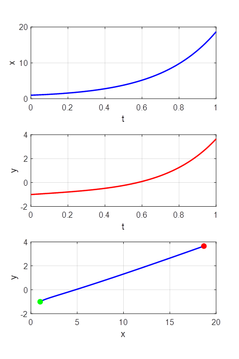
da_RK03.m Sets of First-Order ODEs The Runge-Kutta method can be used to find the solutions of
sets of first-order ODEs. In this example there are
two coupled ODEs. But the method can be extended to
larger numbers of equations. |
|
|
|
|
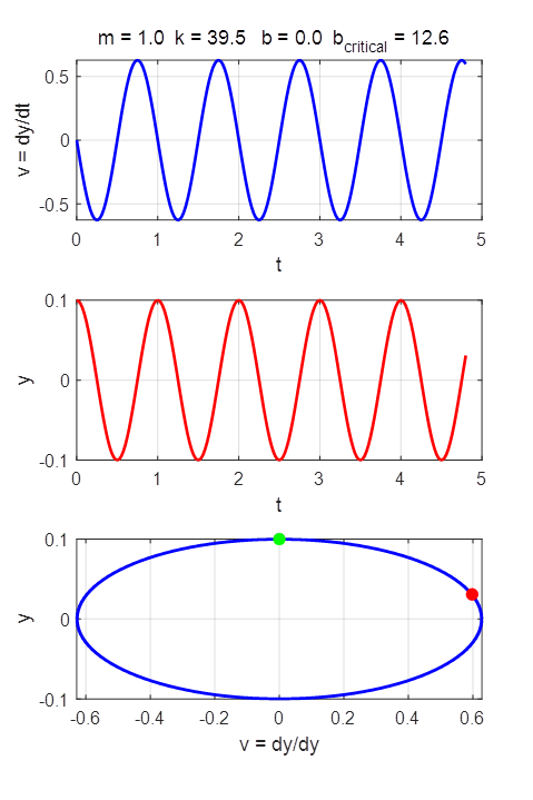
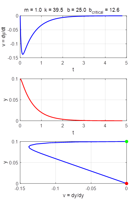
Example 4 da_RK04.m Higher-order ODEs Higher-order ODEs
can be treated as if they were sets of first-order ODEs
(Example 3). We will consider the second-order equation of a damped harmonic
oscillator.
where m is the mass of the oscillator, k is the spring constant, and b is the damping constant. The
variable y(t) is the displacement of the oscillator from the equilibrium position
(y = 0) and v(t) is the velocity of the oscillator The period of oscillation is The constants m, k and b and the initial conditions can be
changed in the INPUT section of the Script. We make the substitution The solutions of the ODE by the Runge-Kutta method for different input parameters are
shown in the following figures: NO DAMPING
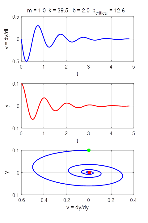
UNDERDAMPING
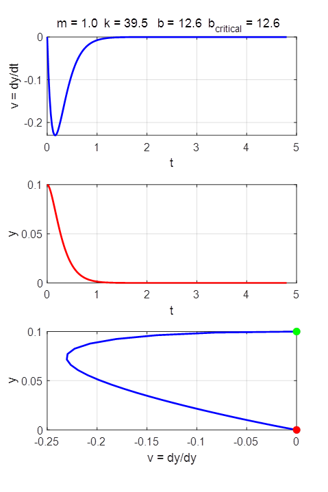
CRITICAL DAMPING (shortest time to
equilibrium with)
OVERDAMPED
|