|
A VISUAL APPROACH:
COMPLEX NUMBERS AND THE FOURIER TRANSFORM John Sims Biomedical
Engineering Department Federal
University of ABC Sao
Bernardo Campus Brazil john.sims@ufabc.edu.br Ian Cooper matlabvisualphysics@gmail.com MATLAB
SCRIPTS / DOWNLOAD DIRECTORY FOR MATLAB SCRIPTS mathComplex4.m Animation of the phase
portrait of the compound complex function for a given winding frequency. mathComplex4A.m Graphical views of a signal function
and the associaed complex exponential finction and the compound complex
function which forms the integrand of the Fourier tranform integral. mathComplex4B.M Calculation of the frequency spectrum
from the variation with winding frequency of the compound complex function. How
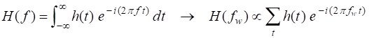
does the Fourier transform relate to complex numbers? On many occasions in science and engineering, we would like to be able to take a signal which varies in time and determine the frequencies contained within it. A well-known approach is to use the Fourier
transform. Fourier transform methods are used in
a very large class of computational problems. Many physical processes can be
described in the time domain by the values of a function (1A) (1B) The integrand is a product of a signal function and a complex exponential function. While the formulae for this transform are available in many books, the student is sometimes without intuitions to understand the mathematics at a deeper level. So, to have a better understanding of the Fourier transform, we need to have a good understanding of complex numbers and by using a visual approach we can understand how the Fourier transform can find the frequency components of the signal function. The inspiration for a visual approach to the Fourier transform came from viewing the youtube video “But what is the Fourier Transform? A visual Introduction” by 3Blue1Brown https://www.youtube.com/watch?v=spUNpyF58BY Matlab programs were developed to create similar figures and to connect the ideas presented in a more formal way with concepts found in a Physics or Electrical Engineering curriculum. It is hoped that the interested student will be able to inspect or modify the Matlab codes that can be downloaded and thereby obtain a deeper understanding of the Fourier transform. COMPLEX NUMBERS AND THE FOURIER TRANSFORM Any complex number can be
expressed in the form
(1)
real part
imaginary part
absolute
value (magnitude)
argument
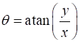
(phase) For each angle To better understand complex functions, we can plot a complex function as a function of time, plot a phase portrait (argand diagram: real part vs imaginary) and use animation effects. The Fourier transform is given by equation 1A (1A) and the inverse Fourier transform is given by equation 1B
(1B) We what to
find the frequency spectrum of the signal function (2) where Therefore,
the integrand (3) One can
gain insight to how the Fourier transform identifies the frequency components
making up a signal by plotting the phase portrait of the compound complex
function
Therefore,
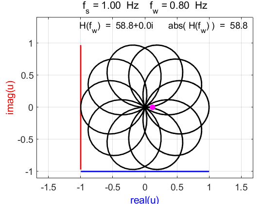
to estimate a frequency component The scripts mathCompex4.m (animations), mathcomplex4A.m (single winding frequency) and mathComplex4B.m (frequency spectrum) are used for the following examples. Minor changes may be necessary in the script to get the best and accurate results. For example, the number of iterations and simulation time may need to be changed. Different signal functions can be used by adding or changing the scripts. You need to adjust the simulation time interval tMax in the script to get a closed and complete trajectory. The best values for tMax maybe 1/fw, 2/fw, 3/fw, … in the script mathComplex4A.m. Example 1 Signal function:
Complex
exponential function:
Compound
complex function:
Fig. 1A. Phase portrait animation of the
compound complex function mathComplex4.m
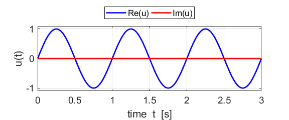
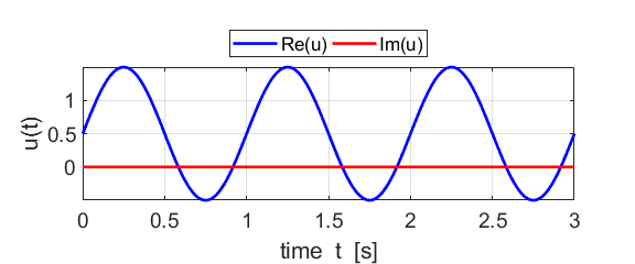
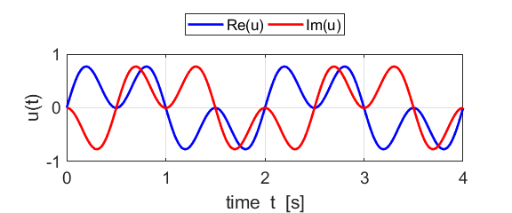
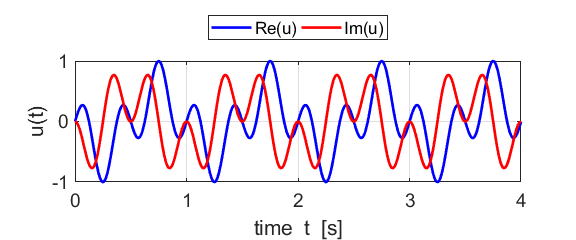
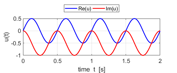
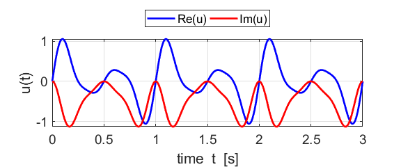
Fig. 1B. The real and imaginary parts of
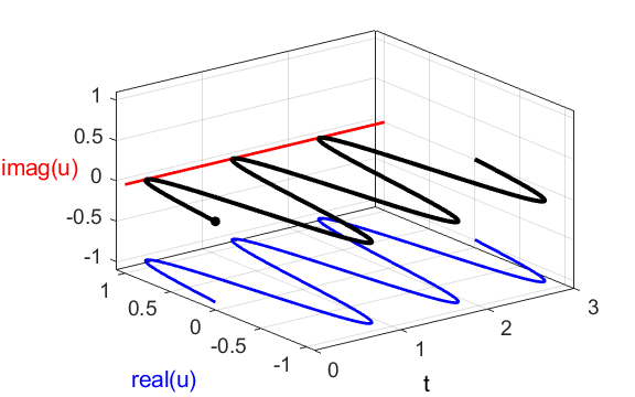
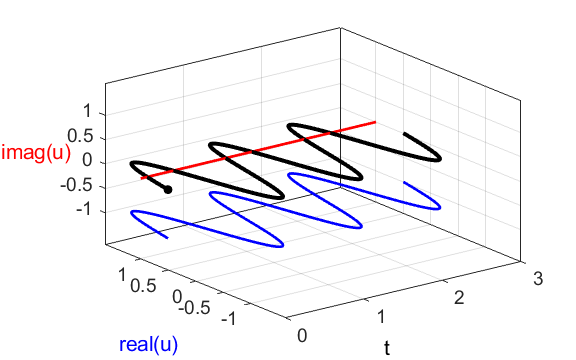
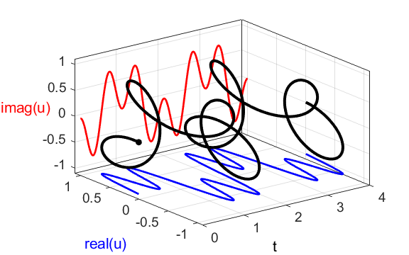
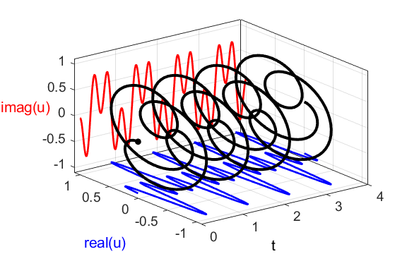
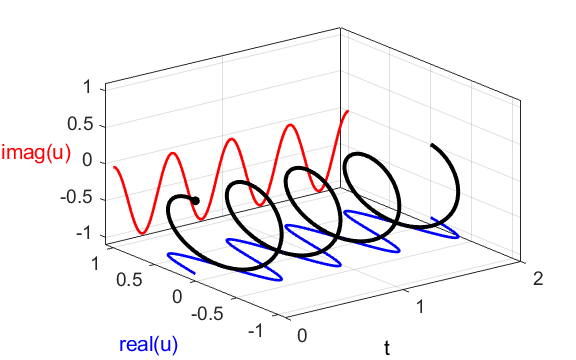
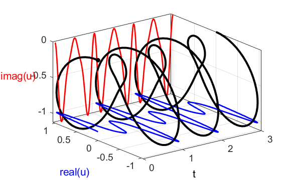
the compound complex function We can also show a [3D] plot of
the time dependence of the compound complex function
Fig. 1C. [3D] view
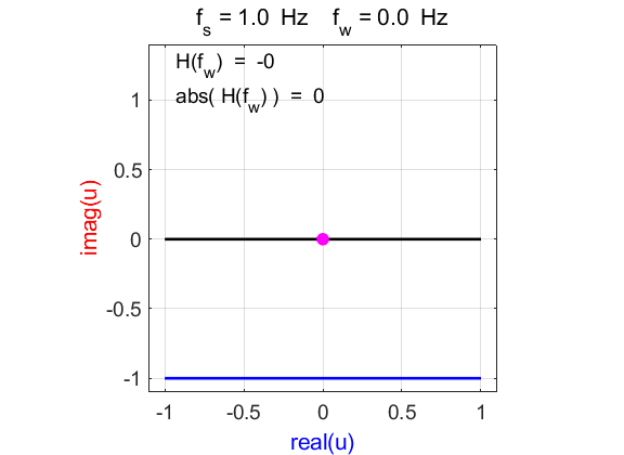
of the compound complex function We can view figure 1C from another
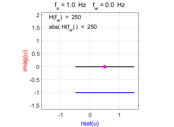
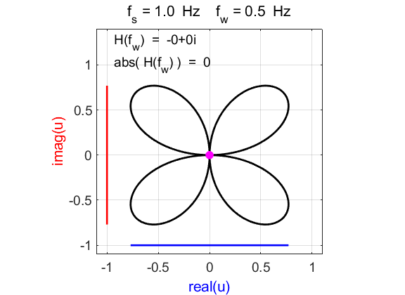
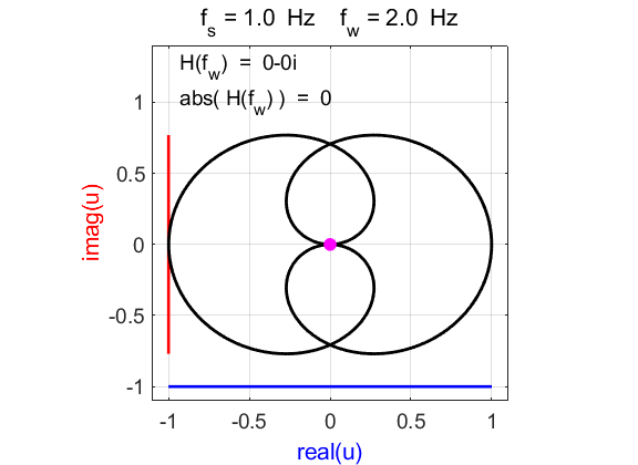
perspective by looking at a plot in phase space which
is the “head-on” view along the time axis as shown in figure 1D.
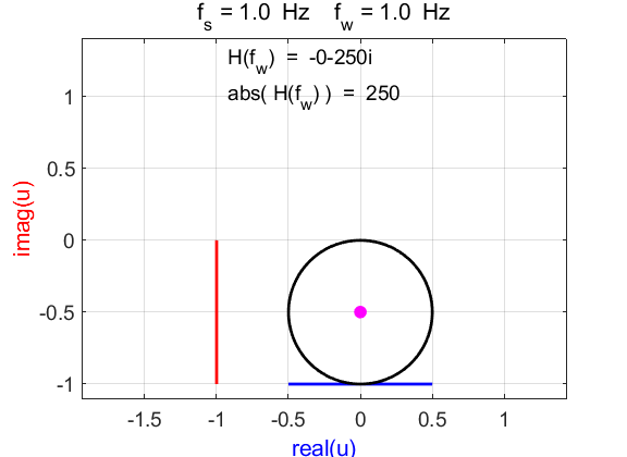
Fig. 1D. Phase plot
of the compound complex function The Fourier transform component
(figure 1D) is Example 2 Signal
function:
Complex
exponential function:
Compound
complex function:
Fig. 2A. Phase portrait animation of the
compound complex function mathComplex4.m
Fig. 2B. The real and imaginary parts of
the compound complex function
Fig.
2C. [3D] view of the
compound complex function
Fig. 2D. Phase plot
of the compound complex function The Fourier transform component
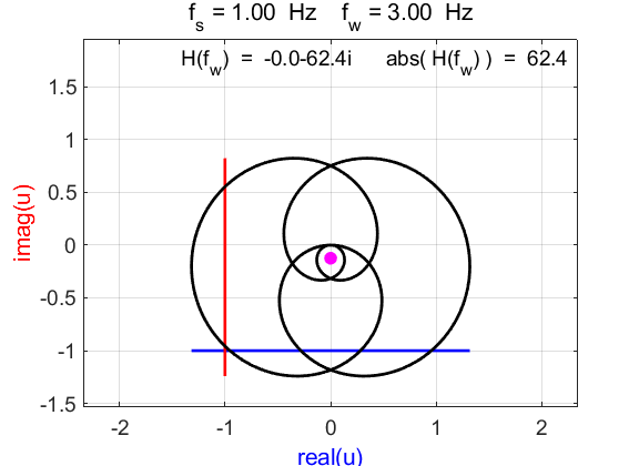
(figure 2D) is Example 3 Signal
function:
Complex
exponential function:
Compound
complex function:
Fig. 3A. Phase portrait animation of
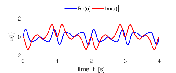
Fig. 3B. Real and
imaginary part of
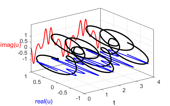
Fig. 3C. [3D] view of Inspection of figure 3C shows why
Fig. 3D. Phase portrait of the function
Example 4 Signal function:
Complex
exponential function:
Compound
complex function:
Fig. 4A. Phase portrait animation of
Fig. 4B. Real and
imaginary part of
Fig. 4C. [3D] view of
Fig. 4D. Phase portrait of the function
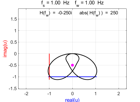
Example 5 Signal function:
Complex
exponential function:
Compound
complex function:
The signal
frequency matches the winding frequency
Fig. 5A. Phase portrait animation of
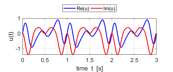
Fig. 5B. Real and
imaginary part of
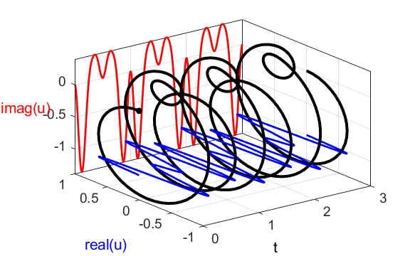
Fig. 5C. [3D] view of
Fig. 5D. Phase portrait of the function
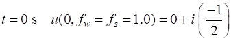
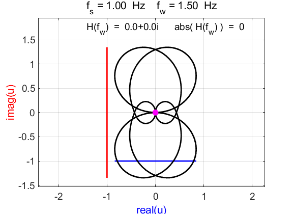
mean(u) à -0.0000 - 0.4990i The
frequency of the compound complex function How do we explain our new plots when We imagine
both f
and If
At time Perhaps
the most interesting feature is that from the point of view of the Fourier
transform, is that the multiplication of the two functions has
resulted in a scaling of the exponential function in the real / imaginary
plane, and a shift
of the centre of rotation from
(0 + i0) to (0 - i0.5) when Example 6 Signal function:
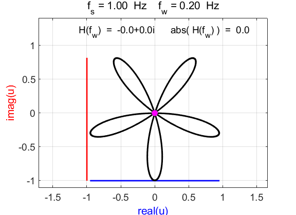
For
winding frequencies not equal to signal frequency
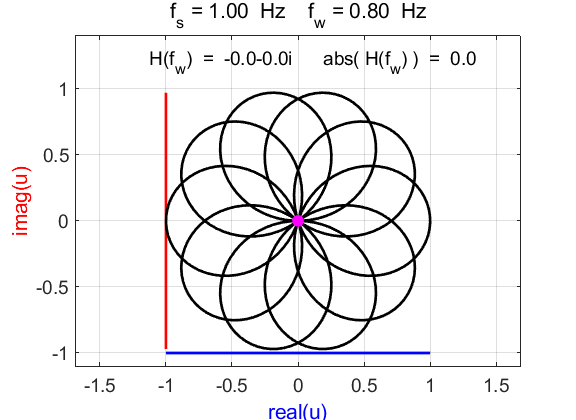
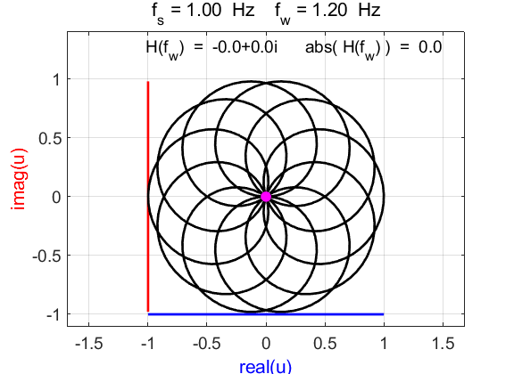
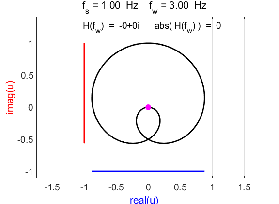
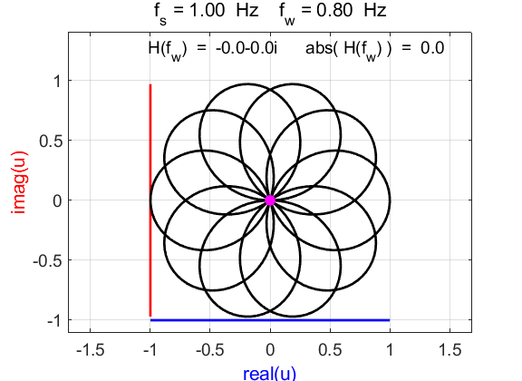
Fig. 6.1. Phase portraits for different
winding frequencies
Fig. 6.2. Phase portraits for winding frequency
Fig. 6.3. Phase portraits for winding frequency From the Command Window, we can calculate the centre position of the trajectory: mean(u)
à 0.1176 + 0.0000i Example 7 Signal function:
Complex
exponential function:
Compound
complex function:
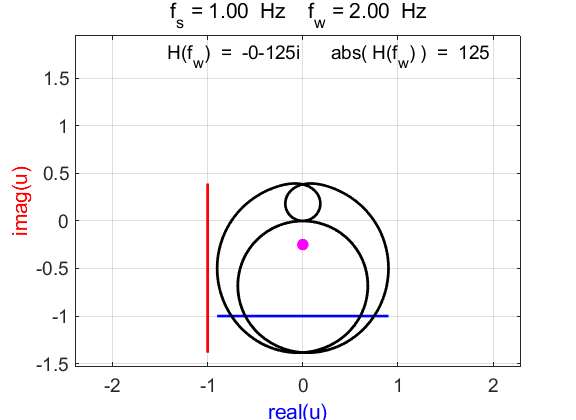
A signal
frequency component matches the winding frequency
Fig. 7A. Phase portrait animation of
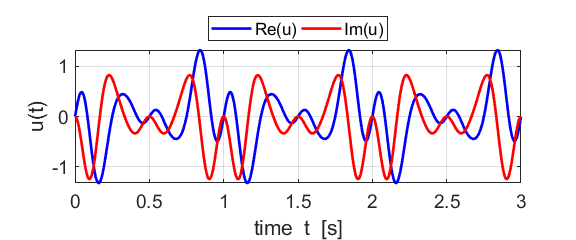
Fig. 7B. Real and
imaginary part of
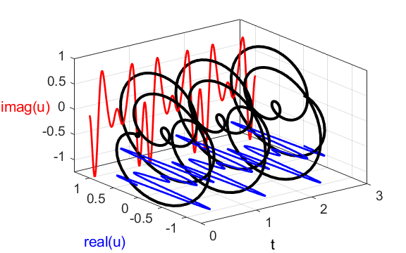
Fig. 7C. [3D] view of
Fig. 7D. Phase portrait of the function A signal
frequency component matches the winding frequency
Fig. 7E. Phase portrait animation of
Fig. 7F. Real and
imaginary part of
Fig. 7G. [3D] view of
Fig. 7H. Phase portrait of the function A signal
frequency component matches the winding frequency
Fig. 7I. Phase portrait animation of
Fig. 7J. Real and
imaginary part of
Fig. 7K. [3D] view of
Fig. 7L. Phase portrait of the function A signal frequency component not matching the winding frequency
Fig. 7I. Phase portrait animation of
Fig. 7J. Real and
imaginary part of
Fig. 7K. [3D] view of
Fig. 7L. Phase portrait of the function When the
winding frequency is not equal to one of the frequency components of the
signal the contribution to the frequency spectrum is zero Signal: Components of signal
(frequency f and amplitude R) and
spectrum contribution
We can clearly conclude that the winding frequency can ‘pick-out’ the spectral components in the signal and give the correct values for the relative amplitudes of each spectral component. FREQUENCY
SPECTRUM OF A SIGNAL
and find its frequency spectrum. The Matlab script maths_ft_01.m was used to find the frequency spectrum of the signal. The graphical output by running the script maths_ft_01.m is shown in figure FT1.
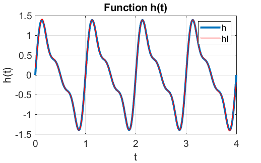
Fig. FT1. The signal function and the inverse Fourier transform.
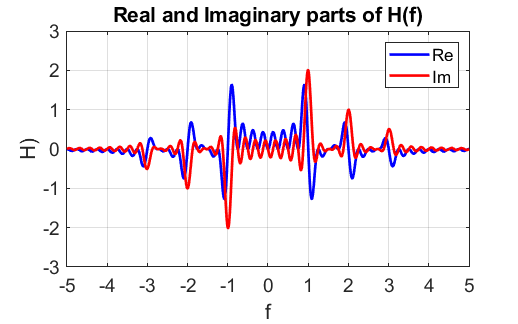
Fig. FT2. The real and imaginary parts of the Fourier transform of the signal.
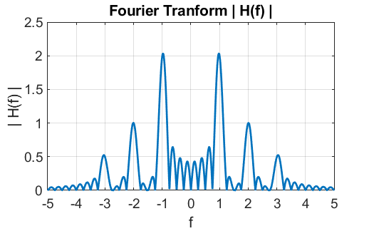
Fig. FT3. The frequency spectrum of the signal. The peaks are at the frequencies 1.0 Hz, 2.0 Hz and 3.0 Hz as expected and the ratio of the peaks are 1 : 0.5 : 0.25 which is in agreement with the relative amplitude of the three sinusoidal functions of the signal
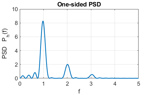
Fig. FT4. The one-sided power spectral
density function Using the script mathcomplex4B.m, we compare the results by performing the Fourier transform using the winding frequencies rather than the direct integration of the integral given in equation 1A.
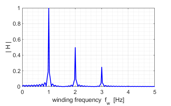
Fig. FT5. The frequency spectrum computed from the winding frequency. The peaks and their heights are as the expected. The wobbles between the peaks arises because at those driving frequency, the stimulation time is such that the last trajectory loop is not completed and so the phase portrait is not symmetrical with a small shift in the centre of the trajectory from the Origin. mathComplex4B.m
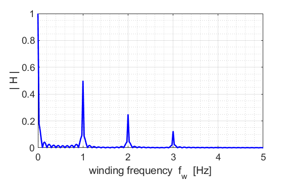
Fig. FT6. The frequency spectrum which has a DC component.
|