|
ORDINARY
DIFFERENTIAL EQUATIONS ode45 RESONANCE: DRIVEN,
DAMPED HARMONIC MOTION van der Pol
Oscillator DOWNLOAD DIRECTORY
FOR MATLAB SCRIPTS https://github.com/D-Arora/Doing-Physics-With-Matlab/tree/master/mpScripts
https://drive.google.com/drive/u/3/folders/1j09aAhfrVYpiMavajrgSvUMc89ksF9Jb math_ode_04.m The Script can be used to help you write your own code in using the Matlab ode solvers for second-order ordinary differential equations. There is a suite of Matlab ode functions which are suitable for just about any type of problem. As an example, the function ode45 is used to solve the equation of motion for a driven-damped mass/spring system. The ode45 works better for nonstiff* problems. It may be beneficial to test more than one solver on a given problem. Type help ode45 in the Command Window to see a list of the ode solvers that you may use. The model parameters are assigned in the INPUT section of the Script. The Script can be easily changed so that the inputs are entered via the Command Window or the Script can be saved as a Live-Script. * A stiff equation is a differential equation for which certain
numerical methods for solving the equation are numerically unstable, unless
the step size is taken to be extremely small. It has proven difficult to
formulate a precise definition of stiffness, but the main idea is that the
equation includes some terms that can lead to rapid variation in the
solution. When integrating a differential equation numerically, one would
expect the requisite step size to be relatively small in a region where the
solution curve displays much variation and to be relatively large where the
solution curve straightens out to approach a line with slope nearly zero. For
some problems this is not the case. Sometimes the step size is forced down to
an unacceptably small level in a region where the solution curve is very
smooth. The phenomenon being exhibited here is known as stiffness. https://en.wikipedia.org/wiki/Stiff_equation math_ode_03.m The Script is used to model a forced van der Pol oscillator. ad_001.mlapp
(App
Designer) GUI for
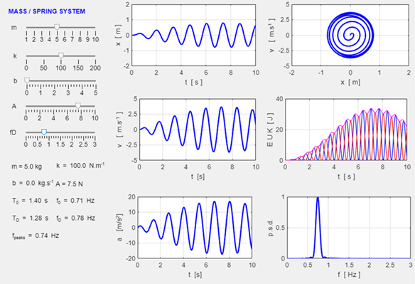
investing the mass spring system
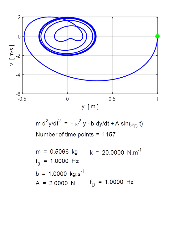
Ordinary differential equations: Initial value problems The Matlab ODE suite of functions computes the time evolution of a set of coupled, first order differential equations with known initial conditions. Such problems are referred to as initial value problems. The function ode45 is an explicit, one-step Runge-Kutta medium order solver which is most suitable for nonstiff problems that requires moderate accuracy. This is typically the first solver you might implement on a new problem. We will use the example for a driven, damped mass/spring system to illustrate the implementation of solving the equation of motion using the function ode45. The equation of motion for the mass/spring system is (1A) (1B) mass m
spring constant k damping constant b
resonance frequency
amplitude of driving force
A frequency
of driving force
displacement
velocity
acceleration
The equation of motion given by equation (1B) for the second derivative must be coded as function. The inputs to this function are the variables t (time), u (displacement and velocity) and K (model parameters). The equation of motion (1B) is expressed as
(1C) where
This function returns the values for the first and second derivatives du and is written as function du = FNode(t,u,K) y = u(1); yDot = u(2); du = zeros(2,1); % First
derivative dy/dt du(1) =
yDot; % ODE:
Second derivative
d2y/dt2 du(2)
= K(1)*y + K(2)*yDot + K(3)*sin(K(4)*t); end The function may not necessarily use the input argument t and output du must be a column vector for the first and second derivatives. The single array K is used as one of the input arguments to the function for the model parameters rather passing on multiple variables. For other differential equations, you will need to change only the values assigned to the array K and change the expression for du(2). The function ode45 is used solve the differential equation as follows: · Define the time interval tSpan which specifies the integration time interval. tSpan = [0 20] gives a time interval from 0 to 20. The number of time steps is determined by the relative tolerance used. The time increments may not necessarily be equal in value. tSpan = linspace(0,20, 1001) gives an integration time of 20 with 1001 equal time increments. · Define the initial conditions as a two-element column vector u0. Initial Conditions (t = 0): displacement is u0(1) and velocity is u0(2).
u0 = [0; 0.5]; · Set the relative tolerance RelTol variable for all solution components. The smaller the relative tolerance, then the more accurate the solution and the greater number of time points.
RelTol = 1e-6;
options
= odeset('RelTol',RelTol); ·
Solve the differential equation using the function ode45.
[t, SOL] =
ode45(@(t,u) FNode(t,u,K), tSpan, u0, options); The
output variables [t, SOL] are time t and SOL where SOL(P:,1) gives
the displacement y
and SOL(:,2) gives
the velocity dy/dt. The acceleration is found using a
finite difference approximation. · From the solution, compute the
displacement y, velocity v and acceleration a. % Displacement [m] y = SOL(:,1); % Velocity [m/s] v = SOL(:,2); % Acceleration [m/s^2] nmax =
length(t); a = zeros(nmax,1); a(1) = (v(2)
- v(1))/(t(2)- t(1)); for n = 2 : nmax a(n) = (v(n)-
v(n-1))/((t(n) - t(n-1))); end Modelling the mass/spring system The model
parameters are entered in the INPUT section of the Script, e.g., % INPUTS
=========================================================== % default
values and units
[ ] % mass [
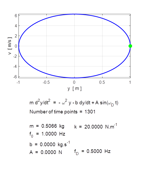
m = 10 kg] m = 0.506606; % spring constant [k = 20 N/m]
k = 20; % Damping constant [b = 2 kg/s] b = 0; % Amplitude of driving force [A = 10 N] A = 0; % frequency of driving force [fD =
1 hz] fD
= 0.5; % Initial conditions [y = 0 m v = 0 m/s] u0 = [1; 0]; % Time span
[0 20 s] tSpan
= [0 10]; % For equal time increments and specify the number of time points
use: % tSpan = linspace(0, 20, 1001); % Relative tolerance for ODE solver [1e-6] RelTol
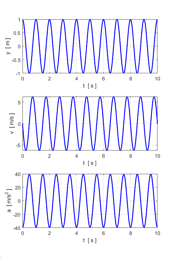
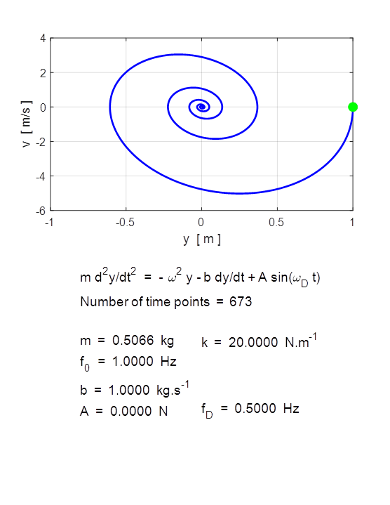
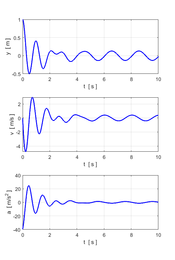
= 1e-6; Free motion
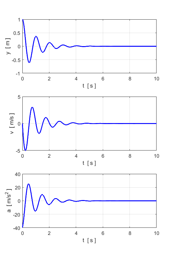
Damped Motion
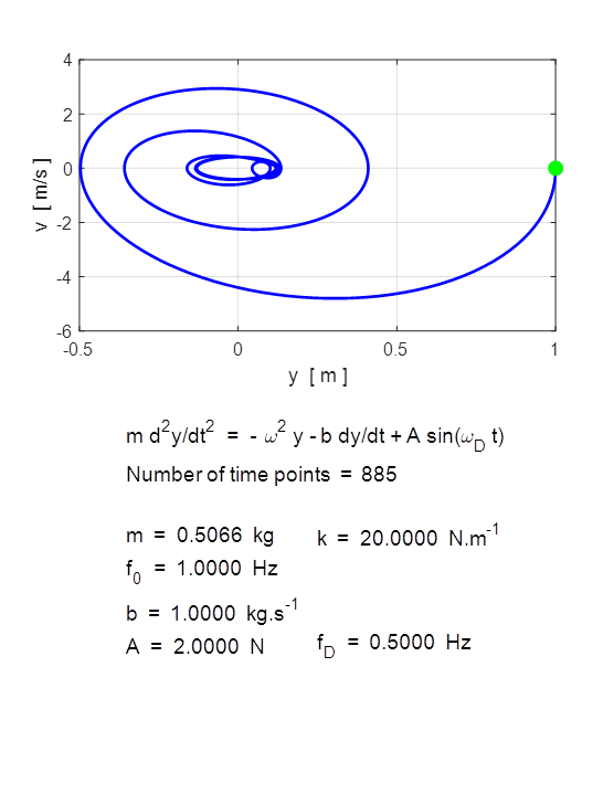
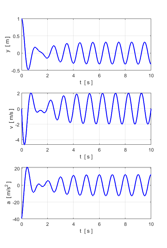
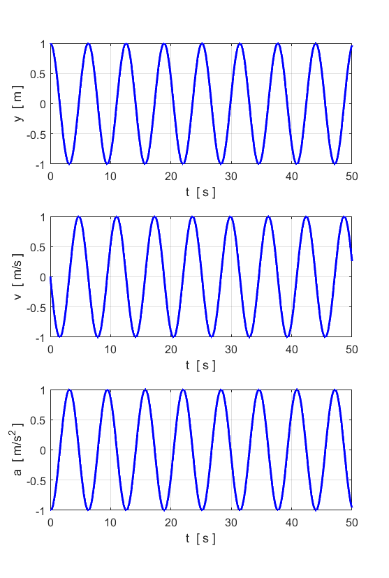
Driven Motion
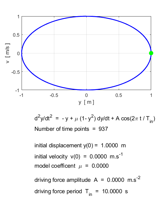
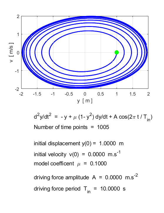
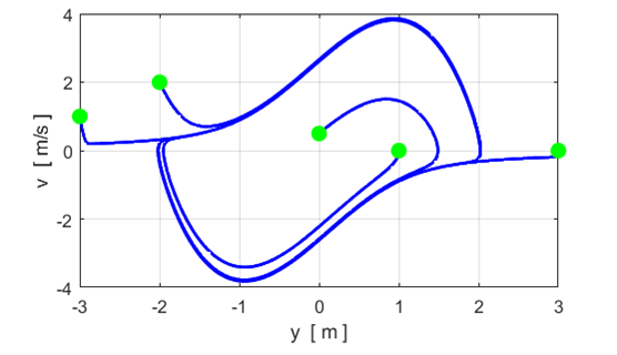
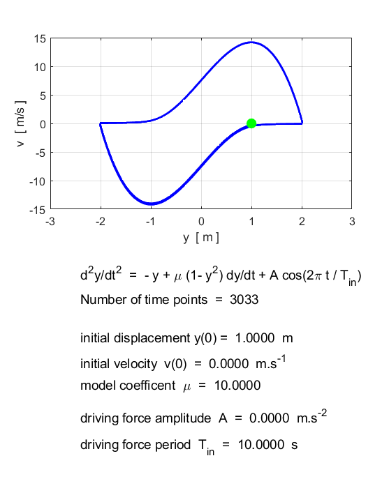
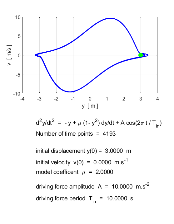
Van der Pol oscillator The
second-order non-linear autonomous differential equation
(2) is called
the van der Pol equation. This form of the van der Pol
equation includes a periodic forcing term and results in deterministic
chaotic motion. The van der Pol equation describes many physical systems. The
parameter The
results of numerical integration of equation 2 are shown below. They show
that for every initial condition (except y = 0, Free motion (simple harmonic motion)
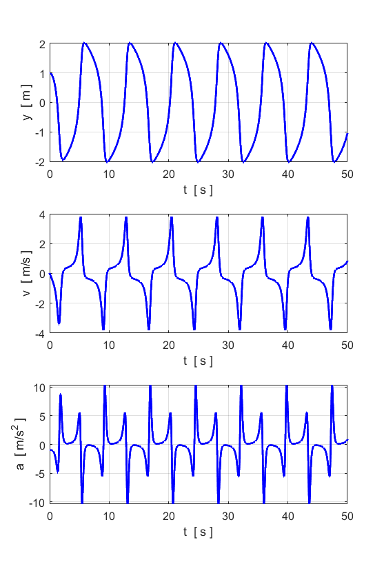
Motion for small values of
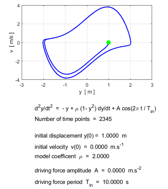
Motion for
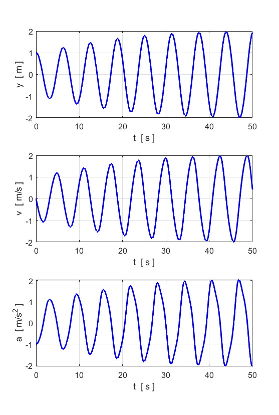
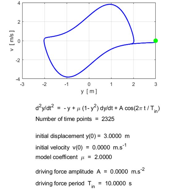
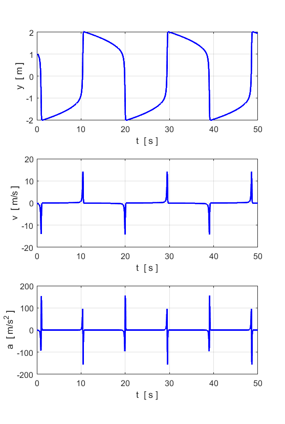
Note: Different initial conditions lead to the same limit cycle. Motion for large values of
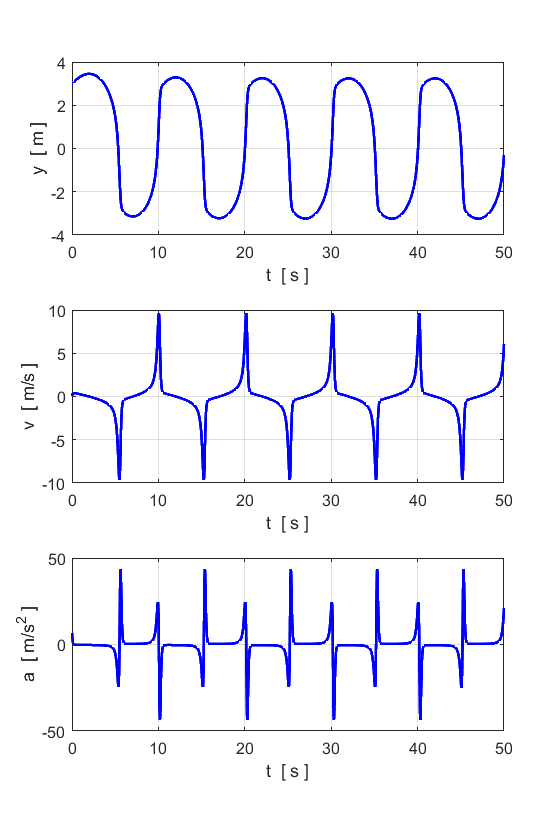
Forced van der Pol oscillator
|
|
|