|
SATELLITE ORBITS: Solving the equation of motion using ode45
|

|
mecSatellite.m An object of mass is
placed into an orbit around a much more massive object of mass M (m << M). It is
assumed the massive object is stationary and the motion of the lighter object
is governed by the Law of Universal Gravitation. The equation of motion of
the lighter object is solved using the function ode45. The initial conditions for the X and Y
components of the displacement and velocity are specified by the parameters
x0, vx0, y0, vy0. The length of the simulation time is specified by tMax and the number of even time increments by nT. Arbitrary units are used for all quantities as GM =
1. |
|
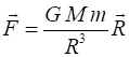
MOTION IN A GRAVITATION FIELD We assume that an
object of mass m is placed into orbit around a
much more massive object of mass M where m << M. The force
between the two objects is given by Newton’s Law of Universal
Gravitation
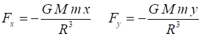
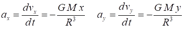
The X and Y components
of this force acting upon the object mass m are and from
Newton’s Second Law, the X and Y components of the acceleration are We can find the
trajectory of the object given its initial conditions at time t = 0
displacement (x0, y0)
velocity (vx0, vy0) The equation of motion
is solved using the Matlab function ode45.
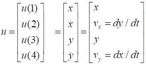
Firstly, we define the column vector u which will give the values of the X and Y displacements and velocity of
the object as function of time
The system of equations is solved using
the function EqM function uDot = EqM(t,u) global GM uDot =
zeros(4,1); R3 = (u(1)^2 + u(3)^2)^1.5; uDot(1) =
u(2); uDot(2) =
-GM*u(1)/R3; uDot(3) =
u(4); uDot(4) =
-GM*u(3)/R3; end The code for the
inputs and for the setup is % Matrix u (X and Y
displacements and velocities) % u(1) = x u(2) = vx u(3) = y; u(4) = vy % Initial
conditions: t = 0 x0 = 1; vx0 = 0; y0 = 0; vy0 = 1.5; % Max time interval
for simulation / number of calculations tMax = 8; nT = 31; % Setup
============================================================== % Earth's radius R_E = 6.38e6; % Earth's mass M_E = 5.98e24; % Universal
gravitation constant G = 6.67e-11; % Mass of
object m = 1; % Use arbitrary
units: Set G*M = 1 % GM = G*M_E; GM = 1; % Initialize u
matrix u0 = [x0 vx0 y0 vy0]; % Time interval:
equal time increments for ode45 tSpan = linspace(0,tMax,nT); options = odeset('RelTol',1e-6,'AbsTol',1e-4); The equations are
solved using the ode45
function over the time interval tSpan starting with the initial conditions
given by u0.
Using the linspace function for tSpan
means that the function is evaluated at fixed time intervals. Many options
for the ode solvers are set via the odeset function. % CALCULATIONS
======================================================= [t,u] =
ode45(@EqM, tSpan, u0,
options); % X and Y
components of displacement and velocity as functions of time t x = u(:,1); vx = u(:,2); y = u(:,3); vy = u(:,4); From the results that
are returned from ode45 function, you can calculate the instantaneous values
for the radius (distance from the Origin), velocity, angular momentum and
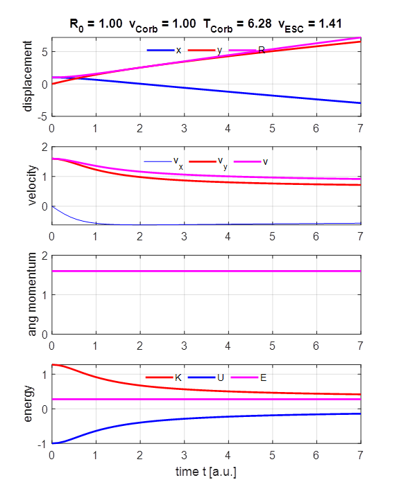
energies (kinetic, potential and total), and the period. % Instantaneous
values
----------------------------------------------- % Radius of orbit R = sqrt(x.^2
+ y.^2); % Velocity v = sqrt(vx.^2
+ vy.^2); % Angular
momentum L = x.*vy - y.*vx; % Energies:
kinetic, potential, total K = 0.5*m.*v.^2; U = - GM*m./R; E = K + U; % Orbital Period
(linear interpolation) flagT = 0; Tindex =
find(y<0,1); if Tindex
> 0 flagT
= 1; mT
= (y(Tindex) - y(Tindex-1))/(t(Tindex)
- t(Tindex-1)); bT
= y(Tindex) - mT*t(Tindex); T = -2*bT/mT; dT
= (t(Tindex)- t(Tindex-1))/2; end Given the initial
conditions, you can calculate the initial radius and hence the period and
orbital velocity for a circular orbit, and the escape velocity. % Circular orbit
------------------------------------------------------ x0 = u0(1); y0 = u0(3); R0 = sqrt(x0^2
+ y0^2); % Orbital velocity vCorb
= sqrt(GM/R0); % Period TCorb
= 2*pi*R0/vCorb; % Escape velocity vESC =
sqrt(2)*vCorb; The trajectory and
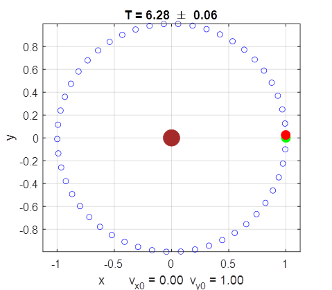
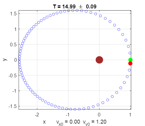
time evolution for the motion are displayed in Figure Windows. SIMULATIONS Circular Orbit
For the circular orbit, the points along the
trajectory are evenly spaced, which shows that the tangential speed is
constant. The green dot shows the starting position and the red dot, the
final position of the object. The numerical estimate of the orbital period
agrees within the uncertainty in its value with the analytical value.
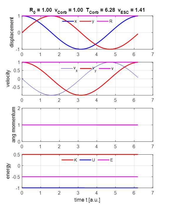
The radius of the orbit is constant. The X
and Y components of the displacement vary sinusoidally.
The magnitude of the tangential velocity is constant and the velocity
components vary sinusoidally. The angular momentum
is constant (Kepler’s Second Law). The
kinetic, gravitational potential energy and total energy are constant. The
total energy is negative at all times. Therefore, the lighter object is bound
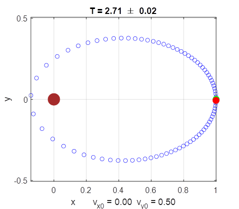
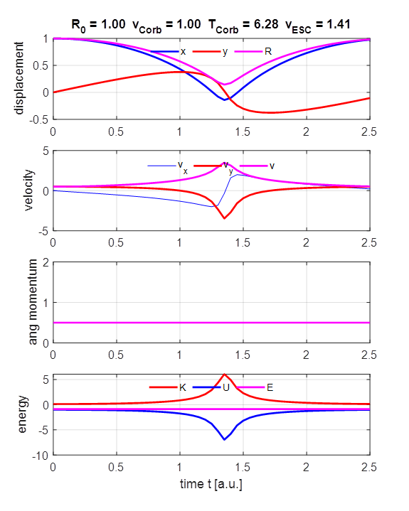
to the more massive object. Elliptical orbit
The orbit is elliptical in shape (Kepler’s First Law). The dots show the position of
the object at even time intervals. At the perihelion (closest point) the dots
are widely spaced indicting a large velocity and at the aphelion (furthest
point) the dots are closely spaced indicating a low velocity. The initial
position corresponds to the aphelion.
The radius of the orbit varies between its
minimum value at the perihelion to its maximum value
at the aphelion. The larger the radius, then the smaller the speed of the
object. The angular momentum is constant (Kepler’s
Second Law). The total energy is constant at all times and negative,
therefore, the lighter object is bound to the more massive object. As the
radius increases in value, the potential energy increases while the kinetic
energy decreases. Elliptical orbit
The orbit is elliptical in shape (Kepler’s First Law). The dots show the position of
the object at even time intervals. At the perihelion (closest point) the dots
are widely spaced indicting a large velocity and at the aphelion (furthest
point) the dots are closely spaced indicating a low velocity. The initial
position corresponds to the perihelion.
The radius of the orbit varies between its
minimum value at the perihelion to its maximum value
at the aphelion. The larger the radius, then the smaller the speed of the
object. The angular momentum is constant (Kepler’s
Second Law). The total energy is constant at all times and negative,
therefore, the lighter object is bound to the more massive object. As the
radius increases in value, the potential energy increases while the kinetic energy
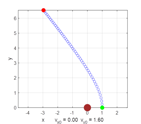
decreases. Escape
The initial speed is greater than the escape
velocity. The object continually moves away from the massive object and can
escape from the influence of the massive object’s gravitational field.
When the lighter object is far from the more massive object, the light object
moves almost with constant speed in a straight line (constant velocity). This
happens because the gravitational force between the two objects decreases
rapidly as their separation distance increases. So, before long the moving
object has effectively escaped the influence of the gravitational attraction.
When the initial vertical velocity is greater
than the escape velocity, the total energy of the system is positive and the
lighter object can escape from the gravitational field of the more massive
object. Comments A circular orbit is
obtained when two conditions are satisfied. (1)
The initial velocity must be directed perpendicular to the line
connecting the initial position to the Origin (0, 0) or centre. (2)
The initial speed must have precisely the value for which the centripetal
acceleration in a circular orbit of radius equal to the initial distance to
the centre which equals the force acting at that distance divided by the mass
of the object. When the initial speed
is higher, the force is not strong enough at that distance to bend the
trajectory into a circle because at that instance its linear momentum is too
large. So, the object starts off on a trajectory which lies outside the
circle. In a single orbit, the object covers a greater distance than in would
in the circular path, thus a longer period compared with the circular
orbit. When the initial speed
is lower than the value leading to a circular orbit, its linear momentum is
reduced, and so the central force is more easily able to change the direction
of motion, bending the trajectory into an orbit inside the circular orbit. In
a single orbit, the object covers a lesser distance than in would in the
circular path, hence, the shorter period compared
with the circular orbit. The reason why the
speed is not constant in a non-circular orbit has to do with the fact that
the force acting on the orbiting object is always directed to the centre at
the Origin (0, 0). Thus, it cannot exert a torque (twist) on it and the
angular momentum of the object must have a constant value. For this to
happen, the object must have a higher speed when it is closer to the fixed
massive object at the centre and a lower speed when it is further away. The motion of the
orbiting object is stated succinctly in Kepler’s
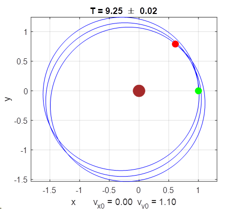
three laws of planetary motion. What happens if the central force slightly deviates from an inverse
square law as described by Newton’s Law of Universal gravitation? Consider changing the
Script temporarily so that function uDot = EqM(t,u) global GM uDot =
zeros(4,1); R3 = (u(1)^2 + u(3)^2)^1.55; uDot(1) =
u(2); uDot(2) =
-GM*u(1)/R3; uDot(3) =
u(4); uDot(4) =
-GM*u(3)/R3; end
The non-inverse square law produces an orbit that
does not close on itself. If you follow with care the orbits, you will
observe that the location on the orbit that is furthest from the Origin
advances, that is, it rotates from one orbit to the next in the same
direction as the rotation of the orbit itself. This phenomenon is called precession. On a very much reduced scale, it is
actually found in planetary orbits. The orbit of Mercury precesses
by about 0.1o per century. This precession is due to the
gravitational effects of the other planets and because the Sun is so massive,
there is a relativistic warping of space in the vicinity of the Sun. Simulation parameters: x0 = 1, vx0 = 0, y0 =
0; vy0 = 1.1,
tMax = 30, nT = 1581 |