|
ALPHA PARTICLE SCATTERING Solving the equation of
motion using ode45
|
Ian Cooper
|
modAlphaSc.m Simulation of an alpha particle scattering
from a positive nucleus of an atom. It is assumed that the nucleus is
stationary. The repulsive force between the alpha particle and the nucleus is
described by Coulomb’s law. The equation of motion of the alpha
particle is solved using the function ode45.
The initial conditions for the X and Y components of the displacement and
velocity are specified by the parameters x0, vx0, y0, vy0. The length of the
simulation time is specified by tMax and the number
of even time increments by nT. Arbitrary units are
used for all quantities as modAlphaScSI.m Similar to modAlphaSc.m Script but
uses S.I. units. The Script can be used to estimate the radius of a uranium
nucleus from the scattering of high energy alpha particles. The impact
parameter is adjusted so that the scattering angle is about 60o.
At this scattering angle, the closest distance of approach of the alpha
particle to the nucleus gives a good estimate of the nuclear radius. |
|
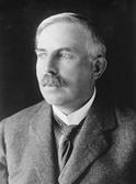
RUTHERFORD: ALPHA PARTICLE SCATTERING
In 1907 Ernst Rutherford in Manchester had the idea to direct alpha
particles produced by the radioactive decay of radium towards a piece of gold
foil, and use the way the paths of these particles were deflected as they
passed through the foil to infer some details about the structure of matter.
The scattering experiments were performed by Rutherford’s assistances
Hans Geiger and Ernest Marsden. The results of the experiment were
unexpected, and Rutherford’s said “It was quite the most incredible event
that has ever happened to me in my life. It was almost as incredible as if
you fired a 15 inch shell at a piece of tissue paper and it came back and hit
you.” Rutherford recognized immediately that the ‘shocking’
Geiger and Marsden result could only be explained if the atom’s
positive charge was not diffuse but concentrated as a small positively charged
core which contained the vast majority of the mass of the atom and with
negatively charged electrons orbiting this positive core. Based on this assumption that most of the mass of the atom lay in a tiny
nucleus, Rutherford worked out an equation to predict how the number of alpha
particles that were deflected to a particular angle should depend on the
energy of the alpha particles and the nature of the target. Geiger and
Marsden performed new experiments which confirmed the predictions of
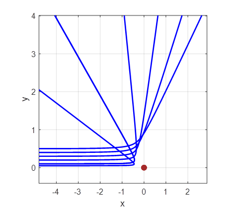
Rutherford’s scattering equation. ALPHA PARTICLE SCATTERING SIMULATION The Script modAlphaSc.m simulates
the scattering of an alpha particle from a stationary positive nucleus. The
result of the simulation shows the trajectory of the alpha particle in a
Matlab Figure Window as shown in figure 1.
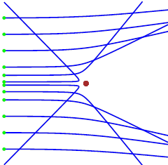
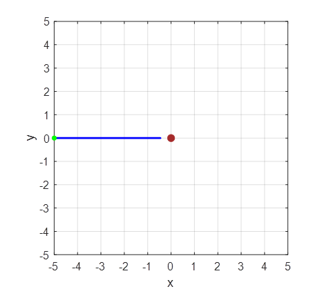
Fig. 1. Simulation of the scattering of
alpha particles from a positive nucleus which is assumed to have a fixed
location at the Origin (0, 0). The statement close is
commented out in the Script and hold on is used for running the Script with different impact
parameters. Arbitrary units are used for all quantities. The greens dot shows the
initial positions of the alpha particles (-5, y0) where y0 corresponds to the
impact parameter. Initially the
alpha particles move to the right with velocity (vx0 = 2 and vy0 = 0). The
alpha particle makes a close collision with the nucleus. The force between
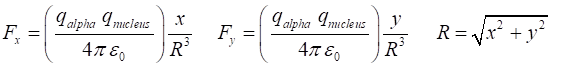
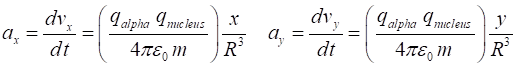
them being the Coulomb repulsion between their positive charges. The X and Y components of this
force acting upon the alpha particle of mass m are and from Newton’s Second
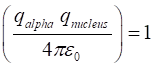
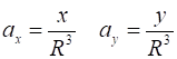
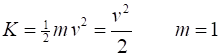
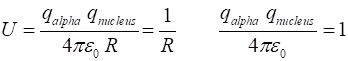
Law, the X and Y components of the acceleration are To simply the calculations, we take m = 1 and let
The equation of motion is solved using the
Matlab function ode45.
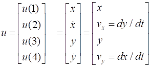
Firstly, we define the column vector u which will give the values of the X and Y displacements and velocity
of the particle as functions of time
The system of equations is solved using
the function EqM function uDot = EqM(t,u) uDot =
zeros(4,1); R3 = (u(1)^2 + u(3)^2)^1.5; uDot(1) =
u(2); uDot(2) =
u(1)/R3; uDot(3) =
u(4); uDot(4) =
u(3)/R3; end The code for the inputs and for
the setup is % INPUTS
>>>>>>>>>>>>>>>>>>>>>>>>>>>>>>>>>>>>>>>>>>>>>>>>>>>>>>>>>>>>>> % Default values % x0 = -5 vx0 = 2 y0 = 1.0 vy0 = 0 % tMax =
8 nT =
181 % Larger values of nT give more accurate results % Matrix u (X and Y
displacements and velocities) % u(1) = x u(2) = vx u(3) = y; u(4) = vy = 0 % Initial conditions: t = 0 % Impact parameter
>>> y0 = 0.1; x0 = -5; vx0 = 2; vy0 = 0; % Max time
interval for simulation / number of calculations tMax = 8; nT = 181; % Setup ============================================================== % Mass of
object m = 1; % Initialize u
matrix u0 = [x0 vx0 y0 vy0]; % Time interval:
equal time increments for ode45 tSpan = linspace(0,tMax,nT); options = odeset('RelTol',1e-6,'AbsTol',1e-4); The equations are solved using the
ode45 function over the time interval tSpan
starting with the initial conditions given by u0. Using the linspace
function for tSpan means that the function is evaluated at fixed
time intervals. Many options for the ode solvers are set via the odeset
function. % CALCULATIONS
======================================================= [t,u] =
ode45(@EqM, tSpan, u0,
options); % X and Y
components of displacement and velocity as functions of time t x = u(:,1); vx = u(:,2); y = u(:,3); vy = u(:,4); From the results that are returned
from ode45 function, you can calculate
the instantaneous values for the separation distance between the charged
particles, velocity, angular momentum and energies (kinetic, potential and
total). % Instantaneous
values
----------------------------------------------- % Radius of orbit R = sqrt(x.^2
+ y.^2); % Velocity v = sqrt(vx.^2
+ vy.^2); % Angular
momentum L = x.*vy - y.*vx; % Energies:
kinetic, potential, total K = 0.5*m.*v.^2; U = m./R; E = K + U; |
|
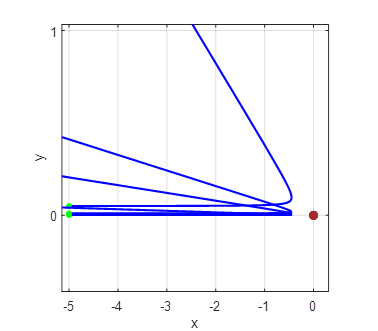
As the impact parameter given by the value y0
gets smaller, the scattering angle becomes larger and for small values of the
impact parameter, the scattering angle is large as shown in figure 2.
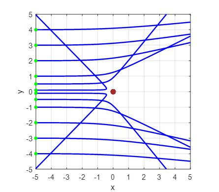
Fig. 2A. Simulation of the scattering of
alpha particles from a positive nucleus which is assumed to have a fixed
location at the Origin (0, 0). Impact parameters (-4, -3, -2, -1, 1, 2, 3,
4)
Fig. 2B. Simulation of the scattering of
alpha particles from a positive nucleus which is assumed to have a fixed
location at the Origin (0, 0). Zoom used to enlarge figure. Impact parameters (0.05, 0.1,
0.2, 0.3, 0.4, 0.5) |
|
|
|
|
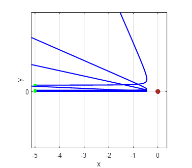
Fig. 2C. Simulation of the scattering of alpha particles from a positive nucleus which is assumed to have a fixed location at the Origin (0, 0). Zoom used to enlarge figure. Impact
parameters (0.001, 0.005, 0.01, 0.05) |
|
|
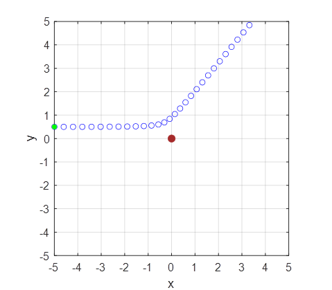
The alpha particle moves to the right at almost constant speed at first
because it is far from the nucleus. As it approaches the nucleus it is slowed
by the repulsion and is thus scattered away from the nucleus and as it
recedes away regaining the speed it had lost (figure 3).
Fig. 3. Stroboscopic properties of the points make what happens during the scattering very apparent. Blue circles are plotted rather than a line: plot(u(:,1),u(:,3),'bo') % plot(u(:,1),u(:,3),'b','linewidth',LW) Figure 4 shows the time evolution of the system for the scattering of the alpha particle. To display the Figure Window in Matlab for figure 4, the variable flag2 is set to 1. % Plot figure
2 (1) yes / (2) no flag2 = 1; if flag2 == 1; close all; end The parameter values for the simulation shown in figures 3 and 4 are: m = 1, y0 = 0.5, x0 = -5, vx0 = 2, vy0 =0, tMax = 6, nT = 31, flag2 = 1
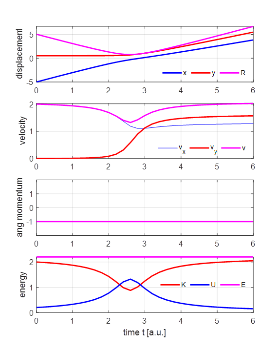
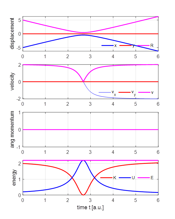
Fig 4. Time evolution of the system. The alpha particle moves towards the nucleus as it slows down and as it recedes it speeds up. The alpha particle is moving at its lowest speed at the point of closest approach. There are zero external forces acting on the positive particles. Therefore, the angular momentum and total energy of the system are conserved in the collision of the alpha particle with the nucleus. As the alpha particle approaches the nucleus, its kinetic energy decreases while the potential energy increases. On receding from the nucleus, the alpha particle’s kinetic energy increases and the potential energy of the system decreases. However, at all times, the total energy remains constant. The kinetic energy of the alpha particle is and the potential energy of the system and its total energy are We can model a head-on-collision by setting y0 = 0 and view the subsequent backscattering. For the initial parameters m = 1, y0 = 0, x0 = -5, vx0 = 2, vy0 = 0, the initial values of the energies are K0 = 2.00, U0 = 0.20 and E0 = 2.20. At the point of closest approach where R = RS, the alpha particle is momentarily stops v = 0. Since the total energy is conserved, the value of the total energy is constant. So, we can estimate the value of the distance of closest approach RS E = E0 =
0 +1/RS = 2.20 The results of the simulation for the head-on-collision are shown in figures 5 and 6
Fig. 5. The backscattering of the alpha particle in a head-on-collision with the nucleus. The distance of closest approach of the alpha particle is 0.4546 which is in excellent agreement with the theoretical prediction of 0.4545.
Fig. 6. The time evolution of the parameters describing the motion of the alpha particle. At the point of closest approach, the speed of the alpha particle is zero. ESTIMATE OF THE RADIUS OF A URANIUM NUCLEUS When alpha particles with 40 MeV kinetic energy
are scattered from uranium nuclei at angles greater than about 60o,
the behaviour of the scattering can no longer be explained by only the
Coulomb repulsive force acting between two nuclei. This implies that when the
two nuclei are close together, the scattering is affected by the overlap of
the strong nuclear force due to each nucleus. You can use the Script modAlphaScSI.m to
estimate the radius of a uranium nucleus. The value of the impact parameters
y0 is adjusted until the angle of scattering is about 60o. Then
the distance of closest approach of the trajectory is the estimate of the
nuclear radius of uranium.
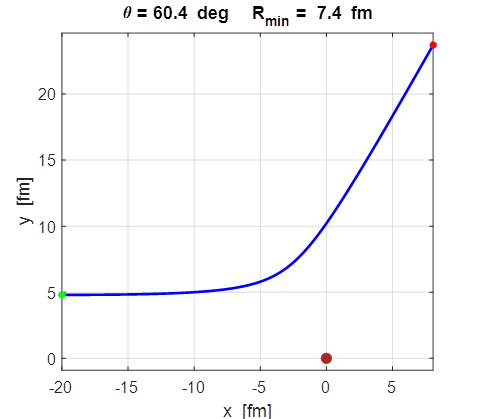
Fig.
7. The impact parameter
y0=4.8x10⁻¹⁵ m = 4.8 fm gives the required scattering angle of 60o.
The distance of closest approach is equal to 7.4 fm. The results of running the simulation for an impact parameter of 4.8 fm gives a scattering angle of 60o and a
distance of closest approach of 7.4 fm. Hence, the estimate of the nuclear
radius of the uranium nuclear is 7.4 fm. The size of a nucleus is often given by the equation
For uranium 235, this equation give a value of 7.4 fm. So, the two
estimates are in good agreement with each other. Figure 8 show the time evolution of the parameters describing the
trajectory of the alpha particle. Since there are zero external forces or
torques acting on the system of the alpha particle and uranium nucleus, both
the angular momentum and total energy of the system are conserved.
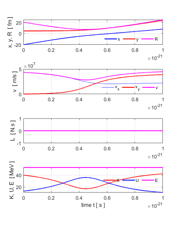
Fig.
8. Time evolution of the
parameters describing the collision of a highly energetic alpha particle and
a uranium nucleus. |
|
|