|
RADIOACTIVITY Solving ordinary differential equations with ode45
|
Ian Cooper
|
modRDecayA.m Simulation: radioactive decay of an unstable
nuclei modRDecayB.m Simulation: radioactive decay of an unstable
nuclei modRDecayC.m Simulation: radioactive decay of unstable
nuclei (nuclear decay chain) Inputs: half-lives, initial numbers of
unstable radioactive nuclei and maximum simulation time. Calculations: The Matlab solver ode45 is used to solve the ordinary differential
equations describing a radioactive decay series. |
|
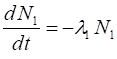
MODELLING RADIOACTIVE DECAY SERIES It is easy solve the ordinary differential
equations describing both single-decay systems and multiple-decay nuclear
chains using the Matlab solver ode45. The fundamental equation is a simple rate
formula. For a single decay of an unstable parent to a stable daughter, the
rate at which the number N1 of nuclei changes with time is
proportional to the number of nuclei itself (1)
where The analytical solution of equation 1 is (2)
where (3)
The solver oder45 is relative easy to setup to solve equation 1
as shown in the Script modRDecayA.m. Figure 1 show the graphical
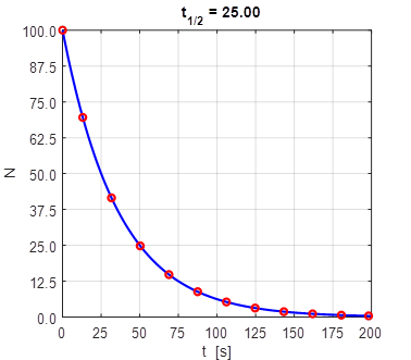
output for the simulation with input parameters t1/2 = 25 s and N0 = 100. Inspection of the plot in
figure 1 clearly shows that the number of nuclei decreases by half in
successive time intervals which equal the half-live value.
Fig. 1.
The radioactive decay of parent unstable nuclei to a stable daughter.
The blue curve is the numerical solution and the red dots the theoretical
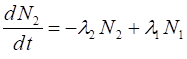
predictions. The next more complicated system allows the daughter to decay
(3)
The analytical solution to this problem is complicated. However, to
solve this problem numerically is easy. The Script modRDecayB.m is used to
solve the coupled differential equations given by equation 3. Sample results
are shown in figures 2,3 and 4.
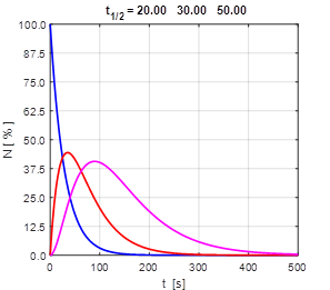
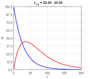
Fig.2. The single decaying daughter
nuclear decay chain. The half-lives of the parent
and daughter have similar values.
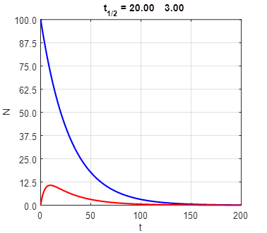
Fig.
3. The half-life of the parent is much larger than the half-life of the daughter. The daughter nuclei decay quickly compared
to their parents. So, the number of daughter nuclei always remains small.
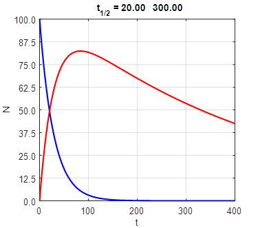
Fig.
4. The half-life of the parent is much smaller than the half-life of the daughter. The daughter nuclei decay slowly compared
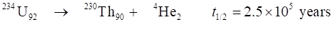
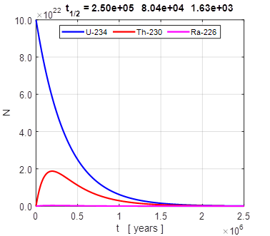
to their parents. So, the number of daughter nuclei can reach large values. It is easy to model long nuclear decay chains. For example, we can
consider the nuclear decay chain for the transformation of 234U92
to lead 206Pb82. The dominant decays are
The Script modRDecayC.m is used to
model the nuclear decay chain for U-234. The results are shown in figures 5A
and 5B. The initial number of U-234 nuclei is 1023 which is about
10 grams.
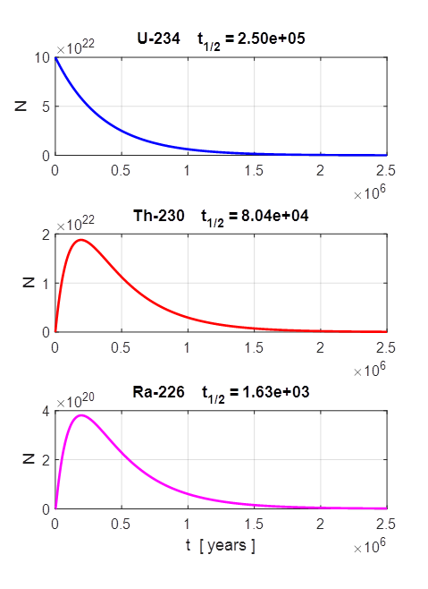
Fig. 5A.
A two-daughter nuclear decay chain:
Fig. 5B.
A two-daughter nuclear decay chain: The number of Em nuclei is essentially the
number of Pb nuclei and is equal to the initial
number of nuclei minus the sum of the numbers of the three decaying dominant
nuclei. So, at any time t
MATLAB SCRIPT modRDecayC.m Input Section: The
variable K gives the values of the decay constant global K % INPUTS
>>>>>>>>>>>>>>>>>>>>>>>>>>>>>>>>>>>>>>>>>>>>>>>>>>>>>>>>>>>>>> % Default values % tH =
100 N0 = 100 tMax = 10*tH % Half-life tH / Initial
number of radioactive nuclei N0 tH(1)
= 2.5e5; N0(1) = 10^23; tH(2)
= 8.04e4; N0(2) = 0; tH(3)
= 1.63e3; N0(3) = 0; % Maximum simulation time tMax =
2.5e6;
Setup Section: % SETUP
=============================================================== % Decay constant
lambda K K = log(2)./tH; % Time interval for
simulation tSpan = [0 tMax]; % Initial
conditions u0 = N0; % Options options = odeset('RelTol',1e-6,'AbsTol',1e-6); % Solve ODE [t,u] =
ode45(@EqM, tSpan, u0,
options); % Undecayed nuclei as a function of time N1 = u(:,1); N2 = u(:,2); N3 = u(:,3); The function for the rate equations describing the decay chain is function uDot = EqM(t,u) global K uDot =
zeros(3,1); uDot(1) =
-K(1)*u(1); uDot(2) =
-K(2)*u(2) + K(1)*u(1); uDot(3) =
-K(3)*u(3) + K(2)*u(2); end
|

|
|