Matlab Physics

HODGKIN – HUXLEY MODEL

FOR MEMBRANE CURRENTS AND ACTION POTENTIALS

Ian Cooper

Email: matlabvisualphysics@gmail.com

MATLAB

npHHA.m

The membrane potential as a function of time of a neuron is calculated using the Hodgkin – Huxley model. A variety of current injection stimuli can be used to view the time evolution of the membrane potential. The stimulus is selected using the variable flagJ. The amplitude of the stimulus is set by the variable J0 where J0 is the maximum current density [A.cm^-2] injected into the neuron.

flagJ = 1 single square current pulse

flagJ = 2 constant current injection: step function

flagJ = 3 double current pulse

flagJ = 4 series of current pulses

flagJ = 5 sinusoidal current stimulus

flagJ = 6 series of current pulses with noise added to each pulse

The model parameters are set within each switch/case section. The differential equations are solved using a finite difference method.

bp_neuron_01bb.m

Data from npHHA.m to plot the spike firing rate against the amplitude of a constant current injection (figure 15).

HODGKIN – HUXLEY MODEL

The core mathematical framework for modern biophysically based neural modelling was developed around 1950 by Alan Hodgkin and Andrew Huxley. They carried out a series of elegant electrophysiological experiments on squid giant neurons which have extraordinarily large diameters (~ 0.5 mm).

Hodgkin and Huxley systematically demonstrated how the macroscopic ionic currents in the squid giant axon could be understood in terms of changes in Na⁺ and K⁺ conductances in the axon membrane. Based on a series of voltage-clamp experiments, they developed a detailed mathematical model of the voltage-dependent and time-dependent properties of the Na⁺ and K⁺ conductances. Their model accurately reproduces the key biophysical properties of the action potential. For this outstanding achievement, Hodgkin and Huxley were awarded the 1963 Nobel Prize in Physiology and Medicine.

In biophysically based neural modelling, the electrical properties of a neuron are represented in terms of an electrical equivalent circuit. Capacitors are used to model the charge storage capacity of the membranes (a semipermeable cell membrane separates the interior of the cell from the extracellular liquid and acts as a capacitor). 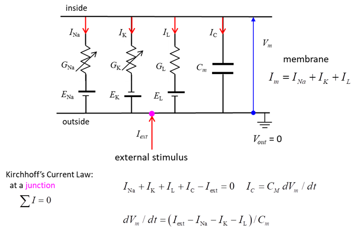Resistors are used to model the various types of ion channels embedded in the membrane, and batteries are used to represent the electrochemical potentials established by differing intracellular and extracellular ion concentrations. Figure 1 shows the equivalent circuit used by Hodgkin and Huxley in modelling a segment of squid giant axon. The current across the membrane has two major components, one associated with the membrane capacitance and one associated with the flow of ions through resistive membrane channels. They found three different types of ion currents: Na⁺, K⁺, and a leak current that consists mainly of Cl^- ions. The flow of ions through a cell membrane of a neuron are controlled by special voltage dependent ion channels: Na⁺ ion channel, K⁺ ion channel and a leak ion channel for all other ions. The neuron can be stimulated by an external current I_ext injected into the interior of the neuron.

Fig.1. Electrical equivalent circuit for a short segment of squid giant axon. Capacitor (capacitance C_m of the cell membrane); Variable resistors (voltage-dependent Na⁺ and K⁺ conductances G_Na, G_K ); fixed resistor (voltage-independent leakage conductance G_L); Batteries (reversal potentials Na⁺, K⁺ , leakage: E_Na, E_K, E_L); Membrane potential V = V_m = V_in - V_out; External stimulus I_ext; Current directions (arrows: I_ext outside ® inside (I < 0), I_Na, I_K and I_L inside ® outside (I > 0).

Conductance G, resistance R ® G = 1 / R.

Electrical activity in neurons is sustained and propagated by ion currents through neuron membranes as shown in figure 1. Most of these transmembrane currents involve four ionic species: sodium Na⁺, potassium K⁺, calcium Ca²⁺ and chloride (Cl^-). The concentrations of these ions are different on the inside and outside of a cell. This creates the electrochemical gradients which are the major driving forces of neural activity. The extracellular medium has high concentration of Na⁺ and Cl^- and a relatively high concentration of Ca²⁺. The intracellular medium has high concentration of K⁺ and negatively charged large molecules A^-. The cell membrane has large protein molecules forming ion channels through which ions (but not A^-) can flow according to their electrochemical gradients.

The concentration asymmetry is maintained through

· Passive redistribution: The impermeable anions A^- attract more K⁺ into the cell and repel more Cl^- out of the cell.

· Active transport: Ions are pumped in and out of the cell by ionic pumps. For example, the Na⁺/K⁺ pump, which pumps out three Na⁺ ions for every two K⁺ ions pumped.

In the Hodgkin – Huxley model only the movement of the sodium, potassium ions are considered, all other ions are considered as part of the leak current.

A mathematical analysis of the equivalent RC circuit for the neuron as shown in figure 1 is outlined by the following equations.

Membrane potential difference measured w.r.t. V_out= 0

(1) V_m = V_in – V_out

Capacitive current: rate of change of charge Q at the membrane surface

(2)

Charge stored on surface of membrane

(3)

Differentiating Q w.r.t. t at a fixed position x₀

(4)

Membrane current due to movement of ions

(5)

Kirchhoff’s current law (conservation of charge)

(6)

The fundamental differential equation relating the change in membrane potential to the currents through the membrane for a small segment of the membrane:

(7) at a fixed position x₀

Equation 7 is better expressed in terms of current density J rather than current I. Dividing equation 9 by an area A, equation 7 becomes

(8) at a fixed position x₀

where

Electrical potential (voltage) DV, current I, resistance R and conductance G are related by the equations

In applying these relationships to ion channels, the equilibrium (reversal) potential for each ion type also needs to be taken into account. This is the potential at which the net ionic current flowing across the membrane would be zero for a given ion species. The reversal potentials are represented by the batteries in figure 1. Hence,

(9)

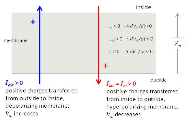
Fig. 3. Sign convention for currents. A positive external current I_ext (outside to inside) will tend to depolarize the cell (i.e., make V_m more positive) while a positive ionic current I_ion will tend to hyperpolarize the cell (i.e., make V = V_m more negative).

In a simple model, the Na⁺ and K⁺ ions are considered to flow through ion channels where a series of gates determine the conductance of the ion channel. The macroscopic conductances of the Hodgkin & Huxley model arise from the combined effects of a large number of microscopic ion channels embedded in the membrane. Each individual ion channel can be thought of as containing one or more physical gates that regulate the flow of ions through the channel. The variation in g values is determined by the set of gate variables n, m and h.

An activation gate ® conductance increases with depolarization

An inactivation gate ® conductance decreases with depolarization

The Na⁺ channel is controlled by 3m activation gates and 1h inactivation gate

The K⁺ channel is controlled by 4n activation gates

From experimental data, the conductances are assumed to described by the following functions

(10)

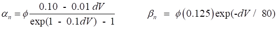
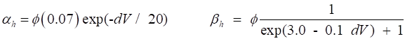
The value of the conductance depends upon the membrane voltage V_m because the values of n, m and h depend on time, their previous value at an earlier time and the membrane potential. The resting membrane potential is given by the symbols V_rest or V_r.

The rates of change of the gate variables are described by the equations

(11)

where the ’s and ’s are rate constants

rate of closed gates opening rate of open gates closing

fraction of gates opening per second

fraction of gates closing per second

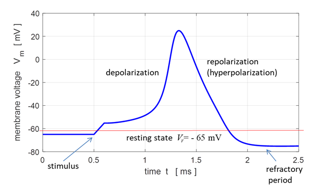
If there is no external stimulus J₀ = 0 and V_m = V_r then J_m = 0 and V_m does not change with time t as dV_m/dt = 0. A stimulus as a result of a current injection into the axon results in the membrane potential either increasing above or decreasing below the resting membrane potential.

The charge per unit area Q deposited into intracellular region by the external stimulus J_ext is given by . If the stimulus is strong enough, an action potential can be evoked as shown in figure 4.

Fig. 4. A strong stimulus to the neuron will evoke an action potential.

The value of the Hodgkin – Huxley parameters used in the modelling are

% FIXED PARAMETERS ====================================================

sf = 1e3; % conversion of V to mV

VR = -65e-3; % resting voltage [V]

Vr = VR*1e3; % resting voltage [mV]

VNa = 50e-3; % reversal voltage for Na+ [V]

VK = -77e-3; % reversal voltage for K+ [V]

Cm = 1e-6; % membrane capacitance/area [F.cm^-2]

gKmax = 36e-3; % K+ conductance [S.cm^-2]

gNamax = 120e-3; % Na+ conductance [S.cm.-2)]

gLmax = 0.3e-3; % max leakage conductance [S.cm-2]

T = 20; % temperature [20 deg C]

NUMERICAL SOLUTIONS OF THE HODGKIN – HUXLEY MODEL

The Script npHHA.m is used to solve equation 8 numerically using a finite difference method to approximate the derivatives.

In this subsection we study the dynamics of the Hodgkin-Huxley model for different types of input which are specified by the variable flagJ.

Single current pulse flagJ = 1

Default input parameters

case 1 % Single current pulse

% Amplitude of pulse [100e-6 A.cm-2]

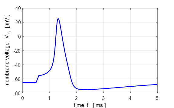
J0 = 100e-6;

% Simulation time [5.0e-3 s]

tMax = 5e-3;

% Time stimulus applied [0.5e-3 s]

tStart = 0.5e-3;

% Pulse duration: ON time [0.1e-3 s]

tON = 0.1e-3;

% Number of grid points [8001]

num = 8001;

If the stimulus is strong enough (sufficient charge injected into the neuron) an action potential will be generated as shown in figure 5.

Fig. 5. Action potential produced by an external current pulse. The time course of the membrane shows the action potential (positive peak) followed by a relative refractory period where the potential is below the resting potential.

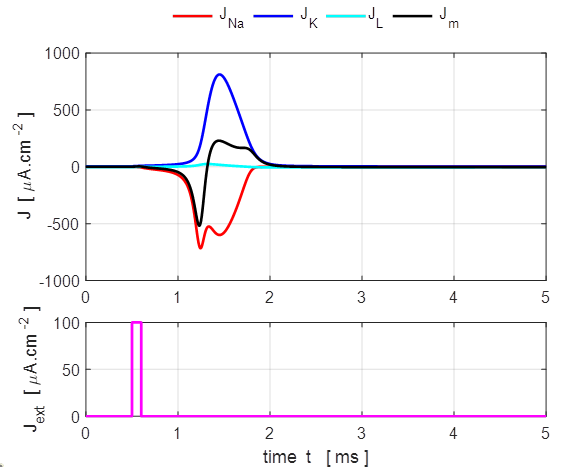
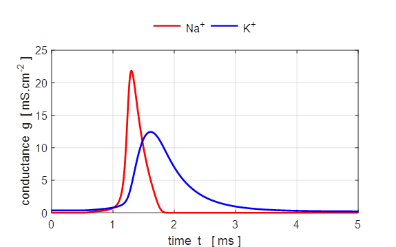
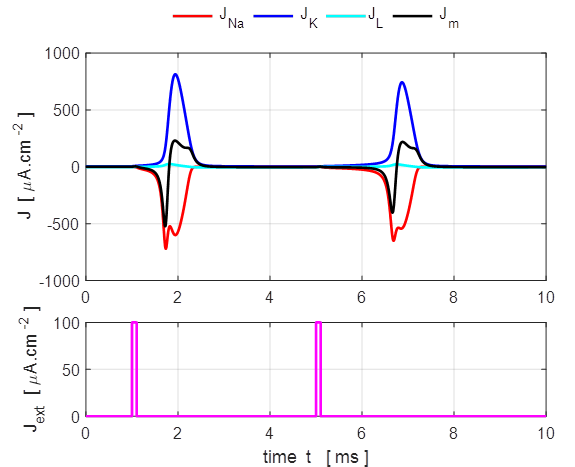
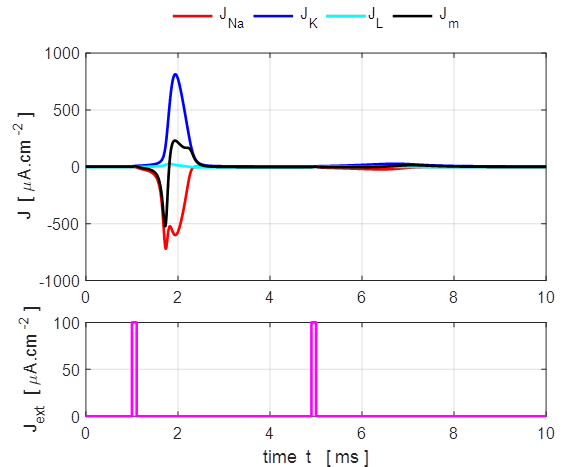
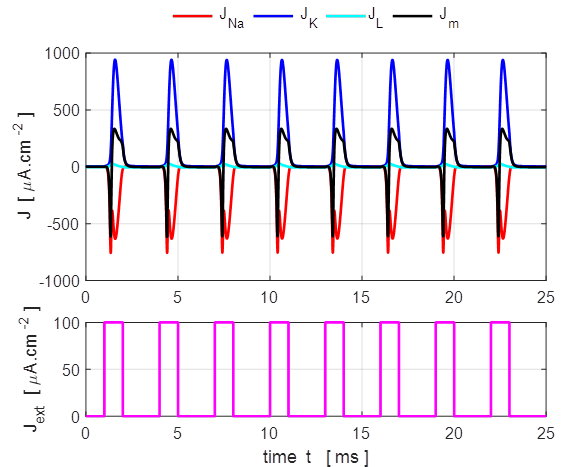
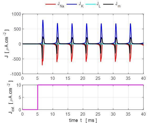
Fig. 6. Only a very small current pulse is required to dramatically change the conductances of the membrane to produce large K⁺ and Na⁺ currents. The potassium current is positive as the K⁺ ions move from inside to the outside of the cell whereas the sodium current is negative as Na⁺ ions move into the cell across the membrane. The Na⁺ and K⁺ currents are nearly balanced throughout most of the duration of the action potential which lasts about 1 ms. The J_Na curve has an extra wiggle around t = 1.3 ms caused by the rapidly changing voltage while the conductance g_Na varies smoothly (figure 7).

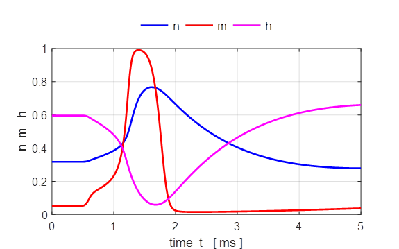
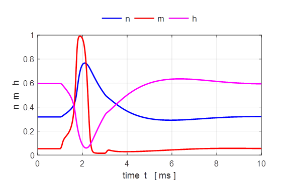
Fig. 7. The gate variables n, m and h and the conductance for potassium and sodium as functions of time. Both the conductances for the Na⁺ and K⁺ ions vary smoothly. The rise in the sodium conductance and fall occur more rapidly for Na⁺ than for K⁺ mainly due to the behaviour of the gate variables m and h. We see that m and n increase with increasing V_m whereas h decreases. Thus, if some external input causes the membrane voltage to rise, the conductance of sodium channels increases due to increasing m. As a result, positive sodium ions flow into the cell and raise the membrane potential even further. If this positive feedback is large enough, an action potential is initiated. At high values of V_m, the sodium conductance is shut off due to the factor h. The time constant for h is always larger than m. Thus the variable h which closes the channels reacts more slowly to the voltage increase than the variable m which opens the channel. On a similar slow time scale, the potassium K+ current sets in. Since it is a current in outward direction, it lowers the potential. The overall effect of the sodium and potassium currents is a short action potential followed by a negative overshoot.

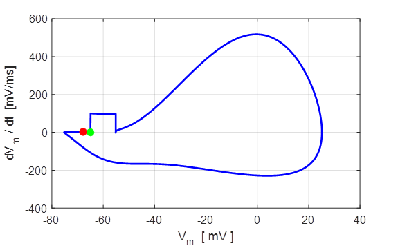
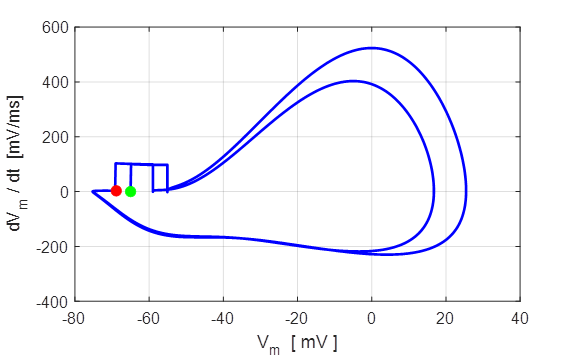
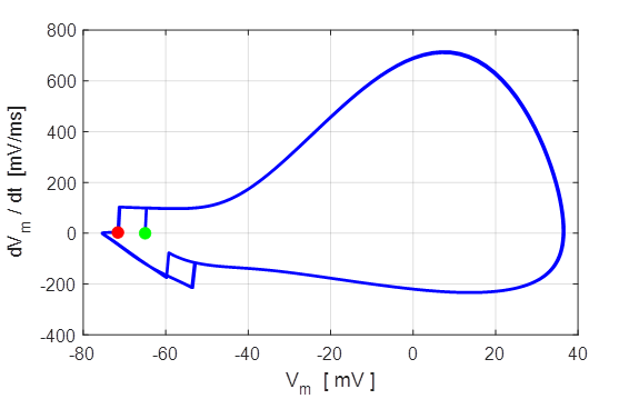
Fig. 8. Phase portrait plot. The membrane potential which equals the rest potential is a stable equilibrium point.

Green dot start (t = 0) and the red dot is finish of the simulation.

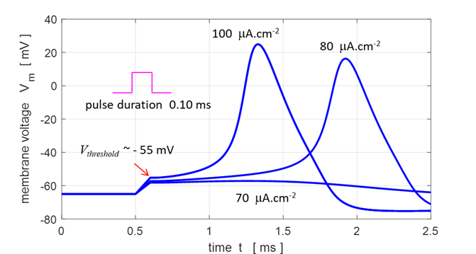
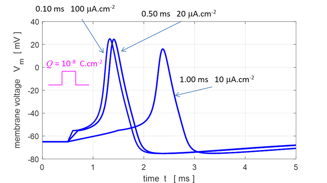
Fig. 9. Membrane responses to three different external stimuli for a square pulse of duration 0.10 ms. J₀= 70 A.cm^-2, no action potential pulse is produced, only a small rise in the membrane potential and then a slow decay back to the resting potential. There is a threshold, when the external stimulus exceeds some critical value an action potential is produced. The threshold is between for the injected current density is between 70 and 80 A.cm^‑2. The action potential rises more rapidly and to a higher peak value when J₀= 100 A.cm^-2 compared with J₀= 80 A.cm^-2. The injected current J_ext acts as a bifurcation parameter. Slight variation in J_ext near the threshold may or may not evoke an action potential.

Fig. 10. The duration and height of the single square pulse is varied such that the charge injected is constant Q = 1.00x10^{-8 C.cm-2}. The pulse with the greatest amplitude and shortest duration produces the action potential which rises most rapidly and with the greatest depolarization.

Fig. 11. A small negative pulse (duration 0.10 ms and height -100 A.cm^-2) causes the membrane potential to be more hyperpolarized before slowly returning to the resting value.

Dual Current Pulses flagJ = 3

We stimulate the Hodgkin-Huxley model by an initial current pulse that is sufficiently strong to excite a spike and a second current pulse of the same amplitude as the
first one in order to study neuronal refractoriness. If the second stimulus is not su
fficient to trigger another action potential, we have a clear signature of neuronal refractoriness.

The response of the membrane potential of two successive square pulses of duration 0.1 ms and amplitude 100 A.cm^-2 are shown in figure 12.

Default input parameters

case 3 % Double current pulse stimulus

% Amplitude of pulses [100e-6 A.cm-2]

J0 = 100e-6;

% Simulation time [2.5e-3 s]

tMax = 10e-3;

% Pulse duration: ON time [0.1e-3 s]

tON = 0.1e-3;

% time pulse #1 ON [1.0e-3 s] / time pulse #2 ON [5.0e-3 s]

t1 = 1.0e-3;

t2 = 5.0e-3;

% Number of grid points [8001]

num = 8001;

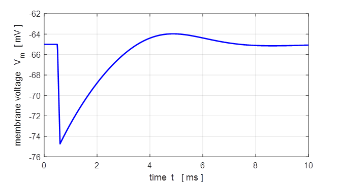
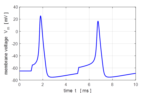
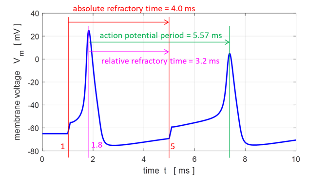
If the time interval between the two pulses is greater than 4.0 ms (t1 = 1.0 ms and t2 > 5.0 ms) then two spikes are generated (figure 12A). When the time interval between pulses is set to 3.9 ms (t1 = 1.0 ms and t2 = 4.9 ms), a second spike is not produced (figure 12B).

Fig. 12A. A second action potential is only produced when sufficient time has passed for the membrane voltage to return to nearly the resting potential. Pulse #1 t1 = 1.00 ms and Pulse#2 t2 = 5.00 ms. Note: in this instance the second spike has a smaller amplitude than the initial spike. not sure if the calculation of refractory times are correct!

Fig. 12B. A second action potential is not produced if there is insufficient time for the neuron to recover. Pulse #1 t1 = 1.0 ms and Pulse#2 t2 = 4.9 ms.

Refractoriness is the fundamental property of excitable medium not to respond on stimuli, if the object stays in the specific refractory state. The refractory period is a period of time during which a neuron is incapable of repeating another action potential. It is the amount of time it takes for an excitable membrane to be ready for a second stimulus once it returns to its resting state following an excitation. The absolute refractory period corresponds to depolarization and repolarization, whereas relative refractory period corresponds to hyperpolarization. The time interval between action potential peaks is 5.57 ms. So, if the neuron was stimulated by a series of square pulses, the maximum frequency of the spikes is about 180 Hz.

Refractoriness occurs, firstly due to the hyperpolarizing spike after-potential which is lower than the resting membrane potential. Hence, more time is needed to reach the
firing threshold. Secondly, since a large portion of the ion channels are open immediately after a spike, the resistance of the membrane is reduced compared to the situation at rest. The depolarizing effect of a stimulating current pulse decays faster immediately after the spike than later (figure 12C).

$Description: D:\mpGateway\npHHA_files\image091.png$

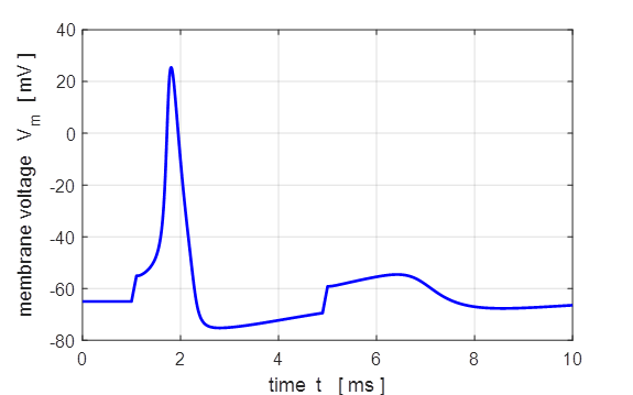
Fig. 12C. The first pulse occurs at time 1.0 ms and the second pulse at 3.0 ms. In the short time interval between the pulses the gating variables have not reached their rest state values. Hence, a large proportion of the ion channels are open.

Multiple current pulses flagJ = 4

You can study the response of the membrane potential to a series of square pulses of uniform amplitude.

Default input parameters

case 4 % Series of current pulses

% Amplitude of pulses [100e-6 A.cm-2]

J0 = 100e-6;

% Simulation time [2.5e-3 s]

tMax = 25e-3;

% Stimulus applied

tSTART = 1e-3;

% Pulse ON / OFF times

tON = 1e-3;

tOFF = 2e-3;

% Number of grid points [8001]

num = 8001;

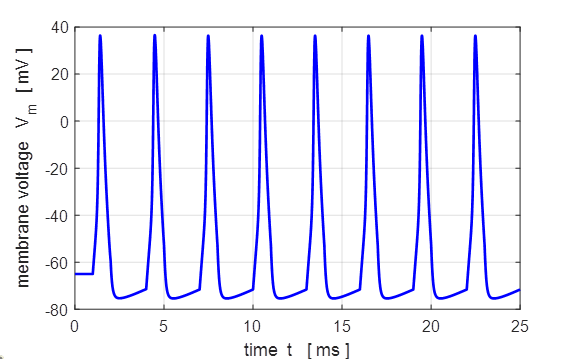
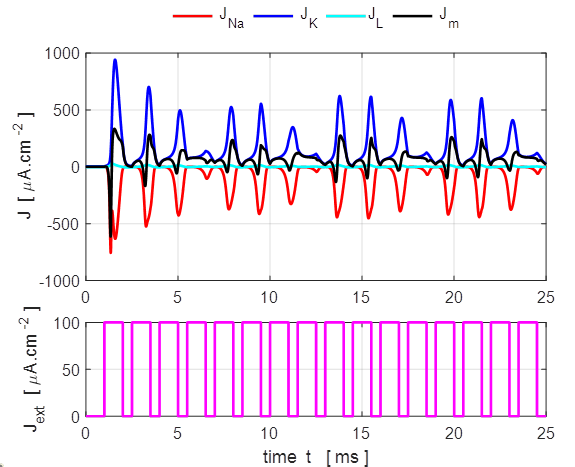
Fig. 13A. The stimulus is applied at time t = 0.1 ms. The pulse amplitude is 100 A.cm^-2. The ON time for each pulse is 0.10 ms and the OFF time is 0.20 ms. A series of regularly spaced action potential are generated. The phase portrait plot shows the limit cycle that describes the dynamics of the system.

Fig. 13B. If the pulse rate is too rapid, then not all action potentials are generated and a regular firing pattern is not established. The simulation parameters for figure 13B are the same as figure 13A except the OFF time of the pulse is reduced to 0.5 ms.

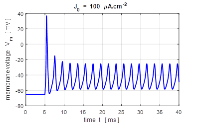
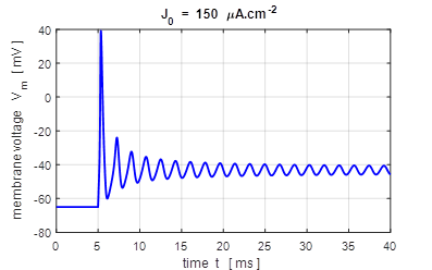
Step current input flagJ = 2

We can model the response of the membrane potential to a step input. Figure 14 shows the membrane potential for a series of step functions with increasing amplitude.

Default input parameters

case 2 % Constant current injection step function

% Amplitude of step function [100e-6 A.cm-2]

J0 = 100e-6;

% Simulation time [40e-3 s]

tMax = 40e-3;

% Time stimulus applied [5e-3 s]

tStart = 5e-3;

% Number of grid points [8001]

num = 8001;

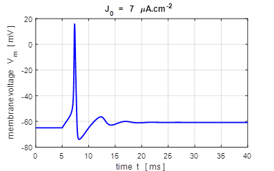
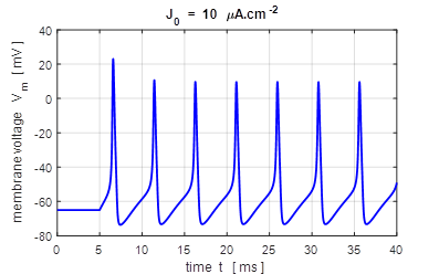
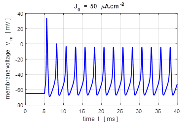
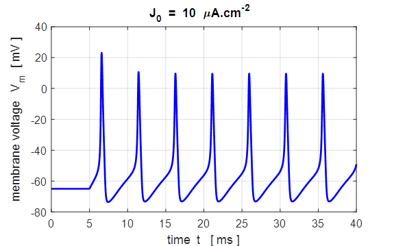
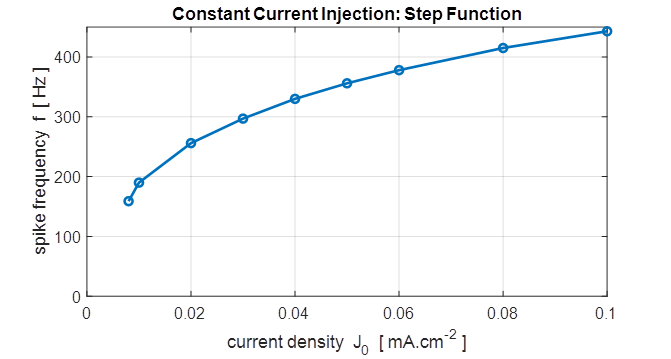
Fig. 14. A constant current injection is used to stimulate the neuron. The stimuli are switched on at time t = 5.0 ms. If the size of the step is less than 7 A.cm^-2 then an action potential is not produced. A current density stimulus of 7 A.cm^-2produces only a single spike. As the size of the step is increased, the frequency of the repetitive firing increases but the degree of depolarization decreases. For the input current density greater than the critical value 7 A.cm^{-2 we} get regular spiking. If the step size is too great, a series of spikes is not produced.

Fig.15A. The frequency f of the repetitive firing was determined for each value of J₀. This frequency is known as the firing rate. The curve is known as the gain function. This was done by using the Matlab command ginput to measure the period of the repetitive firing of the neuron ( inter-spike interval T ) in the Figure Window for the variation in membrane potential as a function of time where f = 1/T . bp_neuron_01bb.m

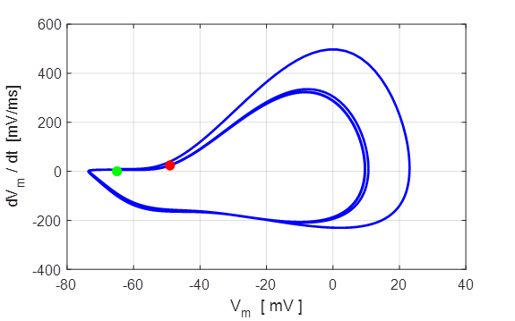
Fig. 15B. The regular spiking of the neuron is clearly shown in the phase portrait plot. The stimulus input current is called a heavy side step function.

Pulse stimulus with noise flagJ = 6

Default input parameters

case 6 % Noise

% Amplitude of step function [7e-6 A.cm-2]

J0 = 7e-6;

% Simulation time [2.5e-3 s]

tMax = 50e-3;

% Stimulus applied

tSTART = 1e-3;

% Pulse ON / OFF times

tON = 1e-3;

tOFF = 2e-3;

% Number of grid points [8001]

num = 8001;

The stimulus corresponds to a series of square pulses whose amplitude is less than the threshold value. Then for each pulse, noise is added using the rand function. A neuron receives signals from thousands of other neurons creating a noisy input resulting in small random fluctuations of the membrane potential around its resting value. The noisy input can lead to a stimulus strong enough to create a depolarization of the membrane producing a spike or a short spike train.

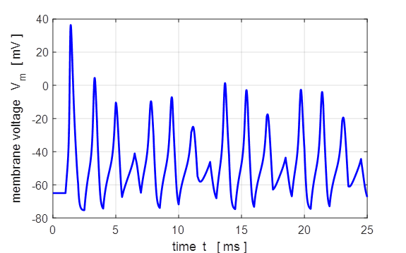
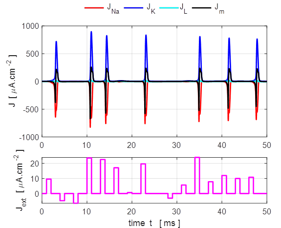
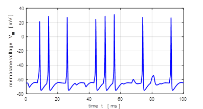
Fig. 16A. Pulse current injection stimulation with noise.

Fig. 16B. The stimulus is a series of injected current pulses with an amplitude less than threshold. Random noise is added to each pulse. A spike train is produced where the spikes are produced spasmodically. Square pulse: J0 = 0.005 mA.cm^-2, tON = 1.0 ms, tOFF = 5.0 ms.

Sinusoidal external stimulus flagJ = 5

Default input parameters

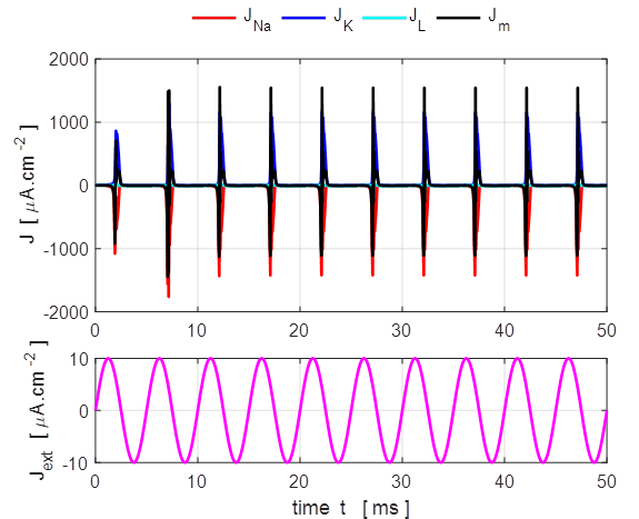
case 5 % Sinusoidal current stimulus

% Amplitude of step function [10e-6 A.cm-2]

J0 = 10e-6;

% Simulation time [50e-3 s]

tMax = 50e-3;

% Frequency of stimulus [200 Hz]

pf = 200;

% Number of grid points [1001]

num = 1001;

The excitation of nerve cells by sinusoidal alternating current waveforms is very dependent upon the frequency of the stimulus because of the necessity to transfer a specific amount of charge to produce the excitation.

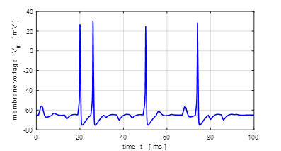
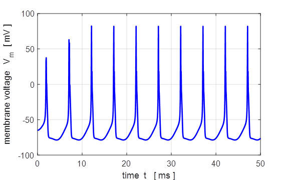
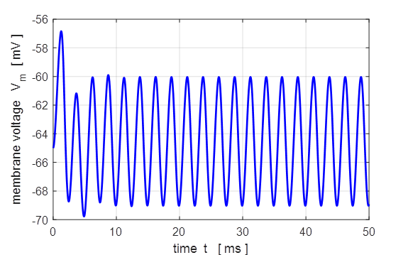
Fig. 17 . A sinusoidal external current stimulus (amplitude 10.0 A.cm^-2, period 5.0 ms and frequency 200 Hz) produces a spike train with a frequency that matches the external stimulus. There is enough time for the membrane of the nerve cell to depolarize as sufficient electric charge can be applied to the membrane within the positive half cycle of the stimulus (charge transferred ).

Fig. 18. A sinusoidal external current stimulus (amplitude 10.0 A.cm^-2, period 2.5 ms and frequency 400 Hz) does not produce a spike train. The membrane potential oscillates with small amplitude around the resting membrane potential (Vrest = - 65 mV) with a frequency that is close to the frequency of the external stimulus. With this higher frequency of external stimulus there is not sufficient electric charge to depolarize the membrane before the current polarity reverses which then acts to repolarize the membrane. From a circuit analysis point of view, there is not sufficient time for the capacitor to charge and hence only a small voltage drop across it can develop. At higher frequency, the impedance of the capacitor is low thus the voltage across it is also low.

The equations of Hodgkin and Huxley provide a good description of the electrophysiological properties of the giant axon of the squid. These equations capture the essence of spike generation by sodium and potassium ion channels. The basic mechanism of generating action potentials is a short in influx of sodium ions that is followed by an efflux of potassium ions. Cortical neurons in vertebrates, however, exhibit a much richer repertoire of electrophysiological properties than the squid axon studied by Hodgkin and Huxley. These properties are mostly due to a larger variety of different ion channels.