DOING PHYSICS WITH MATLAB IZHIKEVICH MODEL FOR ACTION POTENTIALS AND SPIKE TRAINS
Matlab Download Directory ns_Izh002.m Computation of the firing patterns of a single neuron using the Izhikevich Model
This article and the Scripts are based upon the papers by E. M. Izhikevich Which Model to Use for Cortical Spiking Neurons? IEEE Transactions on Neural Networks. Vol. 15. No. 5. September 2004. Izhiekvich’s website Srdjan Ostojic. Two types of asynchronous activity in networks of excitatory and inhibitory spiking neurons. Nature Neuroscience Vol. 17. No. April 2014
Most neurons are excitable in that they can fire a voltage spike when stimulated. In developing useful brain models we want to account for and explain the patterns produced by spiking neurons. To do this we must satisfy two requirements: 1) The model must be computationally simple. 2) The model must be able to produce the rich firing patterns exhibited by real biological neurons. The Hodgkin–Huxley-type models are computationally prohibitive, since they can be used only to simulate a handful of neurons in real time. However, the use of integrate-and-fire models are computationally effective, but the models are unrealistically simple and incapable of producing the rich spiking and bursting dynamics exhibited by cortical neurons. An interesting model to consider was proposed by E. M. Izhikevich. Although this model is not biophysically meaningful, it can be used to compute a wide range of neuron spiking patterns for cortical neurons. The Izhikevich model presented is biologically plausible as the Hodgkin–Huxley model, yet as computationally efficient as the integrate-and-fire model. The value of four parameters a, b, c and d used in the model, determines the spiking and bursting behaviour of the known types of cortical neurons. The time evolution of the membrane potential v is described in terms of the differential equations
(1) (2) The after-spike resetting relationship is (3) where u is the membrane recovery variable.
The dimensions and values of the model parameters are v membrane potential [mV] t time [ms] dv/dt time rate of change in membrane potential [mV.ms^-1 or V.s^-1] u recovery variable [mV] I external current input to cell (synaptic currents or injected DC-currents) [A] c1 = 0.04 mV^‑1.ms^-1 c2 = 5 ms^-1 c3 = 140 mV.ms^-1 c4 = 1 ms^-1 c5 = 1 mV.ms^-1.A^-1
The membrane recovery variable u provides negative feedback to the membrane potential v and accounts for the activation of the K^+currents and inactivation of the Na^+ currents. The term was obtained by fitting the spike initiation dynamics of a cortical neuron so that the membrane potential v has units of mV and the time t is in ms. The model does not have a fixed threshold (as most real neurons) and depending on the history of the membrane potential prior to a spike, the threshold potential may be in the range from -55 mV to -40 mV. The resting potential in the model is between -70 mV and -60 mV depending on the value of the parameter b. Various choices of the parameters a, b, c and d result in the various intrinsic firing patterns that can be computed. a ~ 0.02 ms^-1 determines the time scale of the recovery variable u. The larger the value of a the quicker the recovery. b ~ 0.20 [dimensionless] describes the sensitivity of the recovery variable u to the subthreshold fluctuations of the membrane potential v. Larger values of b couple u and v more strongly resulting in possible subthreshold oscillations and low-threshold spiking dynamics. c ~ -65 mV gives the after-spike reset value of the membrane potential v caused by the fast high-threshold K^+ conductances. d ~ 6 mV describes after-spike reset of the recovery variable u caused by slow high-threshold Na^+ and K^+ conductances. A neuron can be stimulated by the injection of DC current pulse via an electrode and the response of the membrane potential recorded. When a step-input current is used to stimulate a neuron, the neuron continues to fire a sequence of spikes called a spike-train. From such investigations, it is found that neocortical neurons in the mammalian brain can be classified into several firing patterns. Most of these recorded firing patterns can be reproduced computationally using the Izhikevich Model. The following figures show the spike-train patterns for a step input current that causes the neuron to continually fire. The spike-train pattern depends upon the values of the four parameters a, b, c and d and the input current I. The mscript ns_Izh002.m was used to generate the plots. 1. Tonic Spiking and Bursting
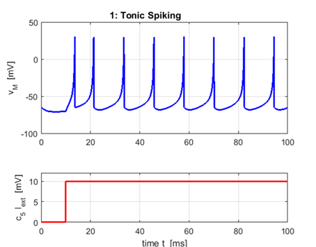
Excitatory neurons: Regular Spiking a = 0.02 b = 0.20 c = -65 d = 6 The most common type of excitatory neurons in the mammalian neocortex are regular spiking cells that fire spikes with decreasing frequency. When presented with a prolonged stimulus the neurons fire a few spikes with short interspike period and then the period increases. This is called spike frequency adaptation. The frequency is relatively high at the oneset of the stimulation and then it adapts. Increasing the strength of the injected DC current increases the interspike frequency, though it never becomes too fast because of large spike after hyperpolarizations.
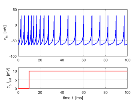
Inhibitory neurons: Fast Spiking a = 0.10 (fast recovery) b = 0.20 c = -65 d = 6 Neurons fire periodic trains of action potentials with extremely high frequency practically without any adaptation (slowing down)
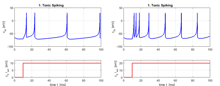
Inhibitory neurons: Low-Threshold Spiking a = 0.02 b = 0.4 c = -65 d = 2 Neurons can also fire high-frequency trains of action potentials, but with a noticeable spike frequency adaptation. These neurons have low firing thresholds, which is accounted for by b = 0.4 in the model. Because of large b value hence low threshold, spikes are produced before external pulse is switched on.
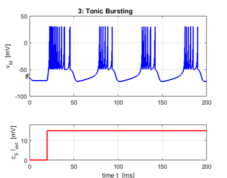
Excitatory (chattering) neurons: Tonic bursting a = 0.02 b = 0.20 c = -50 (very high reset voltage) d = 2 (moderate after-spike jump of u) Some excitatory neutrons such as chattering neurons in a cat cortex fire periodic bursts of closely spaced spikes when stimulated and may contribute to the gamma frequency oscillations in the brain. The interburst frequency can be as high as 50 Hz.
2. Phasic Spiking and Bursting
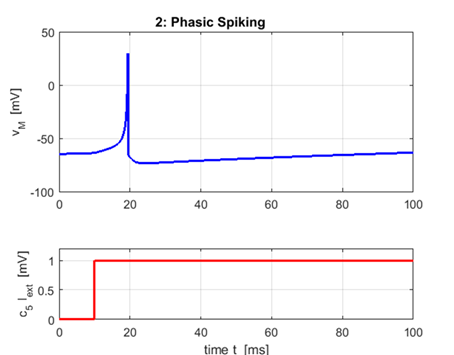
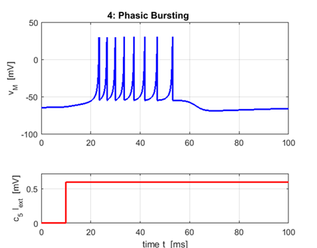
Phasic spiking: a = 0.02 b = 0.25 c = -65 d = 6 A neuron may only fire a single spike at the onset of the input stimulus and remain quiescent afterwards. Phasic bursters: set of closely spaced spikes are generated and then remains quiescent afterwards. a = 0.02 b = 0.25 c = -55 d = 0.05 Phasic bursting importance: · May overcome synaptic failure and reduce noise. · Postsynpatic signal is stronger than that of a single spike. · Selective communication between neurons (interspike frequency within the burst encodes communication channels).
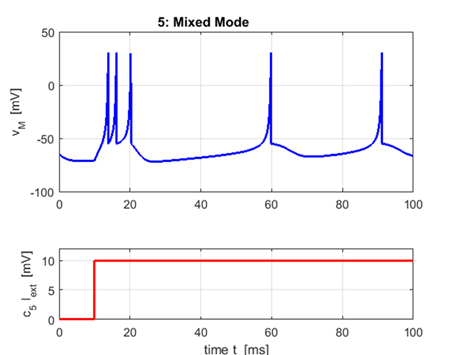
Mixed Mode a = 0.02 b = 0.2 c = -55 d = 4 Excitatory neurons in the mammalian cortex can exhibit a phasic burst at the start of the stimulus and then switch to the tonic spiking mode.
Many more spike-train patterns can be investigated with different input stimulus profiles using the mscript ns_Izh002.m for the Izhikevich Model.