NUMERICAL ANALYSIS OF OPTICAL AND ELECTROMAGNETIC PHENOMENA

POLARIZED LIGHT

MATHEMATICAL FOUNDATIONS

Ian Cooper

matlabvisualphysics@gmail.com

op_005.m

The Script op_005.m can be used to model the any type of polarization. The animations of the electric field vector can be saved as animated gif files (flag1 and flag2). In the INPUT SECTION of the Script, you can enter the amplitudes of the electric field components and their phase angles (flagP = 1) or the Jones parameters (flag2 = 2). From the input values, the electric field (E, Ex, Ey) as functions of time t and position z are calculated. In any plane (z = constant), the electric field vector sweeps out an ellipse with time (a straight line: linear polarization and a circle: circular polarization are special cases of an ellipse). The time evolution of the magnitude of the electric field is used to find its maximum Emax and minimum Emin values and the angle for the orientation of the major axis of the ellipse with respect to the X axis.

switch flagP

case 1

% Relative phase difference of Ey w.r.t. Ex [rad]

phi = phiy-phix;

% JONES VECTOR V and Normalized Jones Vector VN

A = E0x;

B = E0y*cos(phi);

C = E0y*sin(phi);

V = [A; B + 1i*C];

N = sqrt(A^2 + B^2 + C^2);

AN = A/N; BN = B/N; CN = C/N;

VN = V./N;

case 2

E0x = A;

phi = atan2(C,B);

phix = 0;

phiy = phi;

E0y = sqrt(B^2 + C^2);

V = [A; B + 1i*C];

N = sqrt(A^2 + B^2 + C^2);

AN = A/N; BN = B/N; CN = C/N;

VN = V./N;

end

% Time domain

T = 1; % period of vibration [a.u.]

w = 2*pi/T; % angular frequency of vibration [a.u.]

t = linspace(0,T,nT); % time [a.u.]

uT = exp(-1i*w*t); % Wave function for time evolution

% spatial Z domain

k = 2*pi; % Propagation constant

z = linspace(0,3,nZ); % Z domain grid points

uZ = exp(1i*k*z); % Spatial Z wavefunction

% Electric Field

ECx = E0x * exp(1i*phix); % Complex electric field amplitudes

ECy = E0y * exp(1i*phiy);

Ex = ECx .* uT; % time dependent electric field components

Ey = ECy .* uT;

% Magnitude of electric field vector as a function of time

E = sqrt(real(Ex).^2+real(Ey).^2);

% Max magnitude of electric field vector

Emax = max(E);

% Min magnitude of electric field vector

Emin = min(E);

% Index for time when electric field vectro has max magnitude

k = find(E == max(E),1);

% Orientation of major axis of ellipse w.r.t. X axis [deg]

alpha = atand(real(Ey(k))/real(Ex(k)));

% Eccentricity

e = sqrt(Emax^2 - Emin^2);

op_003.m

XY plane animation of a polarized electric field vector for an EM wave propagating in the +Z direction. The electric field is specified by its Jones Vector.

POLARIZED LIGHT

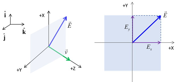
Light is a transverse wave, hence it can be polarized. In the mathematical analysis of polarized light, we only need to consider the electric field and so we can ignore the magnetic field in our description, since the magnetic field can be determined from the electric field via Maxwell’s equations. The electric field is a vector quantity, so we need to specify both its magnitude and its direction. Consider a plane wave propagating in the +Z direction. Then the oscillation of the electric and magnetic fields must be in a XY plane with the electric field perpendicular to the magnetic field. The instantaneous vector representing a ray of light propagating in the +Z direction as shown in figure 1.

Fig. 1. Instantaneous electric field vector of a light ray propagating in the +Z direction. Oscillations of the electric field vector are equivalent to the oscillations of the two orthogonal components and.

The electric field vector can be resolved into two components and directed along the X and Y axes respectively . Then, in terms of unit vectors

Assuming a harmonic variation in the fields, the space and time dependence of the electric field components can be expressed as

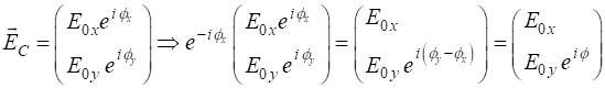
where and are the amplitudes of the components and the phase angles are and . The electric field can now be written as

We can define a complex amplitude and its X and Y components for the electric field

The actual values of the electric field and its components are found by taking the real parts of the complex functions. A convenient way thinking about polarized light is that it is a superposition of two linear polarized components vibrating along the X and Y axes.

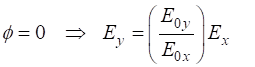
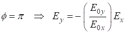
The classification or state of the polarization depends upon the relative phase of the vibrations of the Y component of the electric field with respect to the X component and on the relative amplitudes.

Polarization state (mode) depends on:

In an XY plane, the electric field vector sweeps out an ellipse with time which is enclosed by a rectangle having dimensions . Note: a straight line and a circle are special cases of an ellipse. The eccentricity e of the ellipse depends on the relative phase difference reaching a maximum when and a minimum when .

Increasing or decreasing the relative phase angle by an integer multiple of does not change the state of polarization

STATES OF POLARIZATION

· Linear polarized

vertical polarized

horizontal polarized

straight line through (0,0) with slope > 0

vertical polarized

horizontal polarized

straight line through (0, 0) with slope < 0

· Left Circular polarized

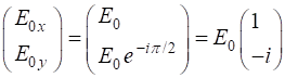
Anticlockwise rotation of the electric field vector in a XY plane

lags by rad or 90^o

The term is used for the phase, so we have to add to the phase of . reaches its maximum value a quarter of a cycle after does.

The electric field vector sweeps out a circle in an anticlockwise sense as viewed head-on looking back along the Z axis. This is referred to as left circular polarized light (positive helicity). For a fixed value of t, the electric field vector describes a spiral on the surface of a cylinder of radius with its axis along Z.

· Right Circular polarized

Clockwise rotation of the electric field vector in a XY plane

leads by rad or 90^o

The term is used for the phase, so we have to add to the phase of . reaches its maximum value a quarter of a cycle before does.

The electric field vector sweeps out a circle in a clockwise sense as viewed head-on looking back along the Z axis. This is referred to as right circular polarized light (negative helicity). For a fixed value of t, the electric field vector describes a spiral on the surface of a cylinder of radius with its axis along Z.

· Elliptical polarized major axis of ellipse aligned along the X axis or Y axis

left elliptical polarization

right circular polarization

· Elliptical polarized

left elliptical polarization

right circular polarization

JONES VECTORS

We can employ a matrix technique developed by R.C. Jones (1941) to give a mathematical description of polarization. A two-element column vector is used to represent light in various modes of polarization.

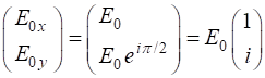
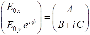
The state of polarization of light is completely determined by the relative amplitudes and relative phase of the components and . So, we only need to consider the complex amplitude and we can write it as a two-element vector (2 element column matrix) or Jones Vector

The X component element of the Jones vector is taken as a real quantity and we can always multiply the column vector by suitable quantity to achieve this. Since the state of polarization only depends upon the relative amplitudes, the multiplication of the column vector by a constant does not change the state of polarization angle.

The most general case for the Jones Vector is expressed as

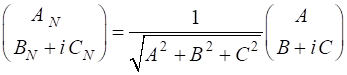
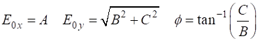
where A, B and C are real constants.

The normalized Jones vector is defined such that

So, given the Jones Vector expressed in terms of A, B and C we can calculate the electric field components and the relative phase

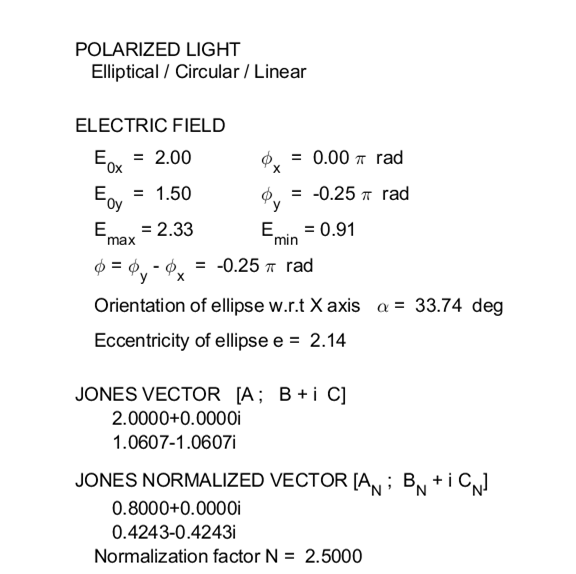
or given the electric field components, we can calculate the Jones parameters A, B and C

EXAMPLE op_005.m

We can illustrate the power of using the Matlab Script op_005.m to investigate the properties of the state of polarization for elliptical light specified by the input values

E0x = 2;

E0y = 1.5;

phix = 0;

phiy = -pi/4;

flagP = 1;

Fig. 2. A Figure Window is used to give a summary of the parameters for the simulation of the propagation of a polarized EM wave. Note: Emax is calculated numerically. The greater the number of time steps the greater the accuracy of the value for Emax. The correct value for Emax is 2.50 and so the value Emax = 2.33 is only an approximation.

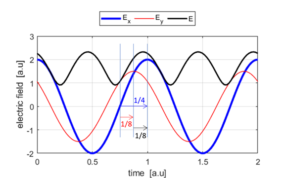
Fig. 3. The time evolution of the electric field for two cycle. The black curve shows the variation in the magnitude of the electric field ; the blue curve shows the X component and the red curve, the Y component . The Y component leads the X component by rad .

Fig. 4. Animation of the elliptical polarized light oriented at an angle relative to the X-axis. The normalized values of the electric field and its X and Y components are shown. The black line shows the instantaneous electric field vector which rotates in a clockwise sense. Hence, the light is right elliptical polarized. The amplitudes of the electric field components are and The magnitude of the electric field vector is The red vertical line shows the Y components of the electric field and the blue horizontal line the X component. You can see that the ellipse is enclosed by a rectangle of sides and where N is the normalization factor.

Fig. 5. Animation of the electric field propagating in the +Z direction. The blue curve shows the X component , the red curve the Y component and the black curve the electric field vector whose path sweeps out an elliptical helix with time. Looking back along the Z axis, the rotation of the electric field vector is clockwise, so the light is right elliptical polarized.