|
NUMERICAL ANALYSIS
OF OPTICAL AND ELECTROMAGNETIC PHENOMENA MODELLING THE
BEHAVIOUR OF GAUSSIAN BEAMS (PARAXIAL REGIME) Matlab Script Download Directory op_beams_001.m The Script is used to model the behaviour
of a Gaussian beam propagating in the Z direction with spherical wavefronts
in the paraxial region. The beam is specified by its wavelength
(visible part of the electromagnetic spectrum), power and
the value of its waist. Also, the XY and XZ planes for the irradiance
calculations and plots are also specified in the INPUT Section of the Script.
The following parameters are computed in the CALCULATION Section of the
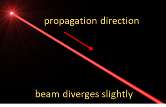
Script: the Z axis grid, INTRODUCTION Lasers are widely used in many fields today. Having a mathematical description of laser light is essential. The light emitted from a laser is composed of a narrow band of wavelengths, such that we can assume the light is monochromatic. The light emitted from the laser is usually collimated as it propagates in a straight line as a narrow beam. As a starting point, we will assume the beam to be unpolarized and the light intensity to have a Gaussian profile in any plane that is normal to the direction of propagation. This mode is referred to as the TEM00 mode and it describes the output of most lasers.
Fig. 1. Red light emitted from a HeNe laser. The light is seen due to scattering. The light propagates as a collimated beam in a straight line with slight divergence in its cross-section. The light emitted from a laser can be
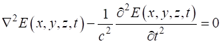
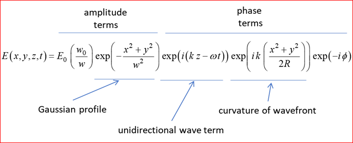
modelled by solving the [3D] scalar wave equation for the electric field
(1) We will assume that a monochromatic beam with a circular cross-section propagates in free spaces and that the electric field can be expressed as a product of its spatial part and time dependent part
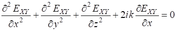
(2) Substitution of equation 2 into equation 1 gives the Helmholtz equation
(3) We will only consider the solution for a wave propagating in the Z direction where
(4) The term Substitution of equation 4 into equation 3 gives
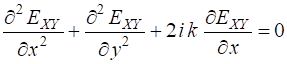
(5) We will assume that there is a slow decrease in the amplitude of the wave as the wave propagates in the Z direction and only consider the wave far from the origin but close to the Z axis such that
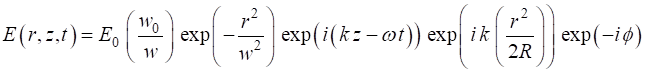
(6) This is known as the paraxial wave equation. Without going into all the mathematical details, a solution to paraxial wave equation is
(7) where
(8)
The paraxial
approximation is only valid when
We can better understand the solution of the scalar paraxial wave equation by running the Script op_beams_001.m with the following input parameters: % INPUTS
============================================================== % Max
power transmitted in beam
[W] P0 = 1e-3; % beam waist [m] w0 = 0.5e-3; % wavelength [m] wL = 632.8e-9; % Length
of Z domain in multiples of zR : z = nZ * zR nZ = 5; % Number
of grid points in calculations (must be an odd number) N = 501; % Z
position of XY plane for radial irradiance plots: zPR = zP / zR % [e,g, zPR = 0, 1, 2, ... ] zPR = 4; % Max
radial distance for radial irradiance plot: Rmax = nR * w0 nR = 5; All the figures in this document where created using the script op_beams_001.m. Beam spot At position z
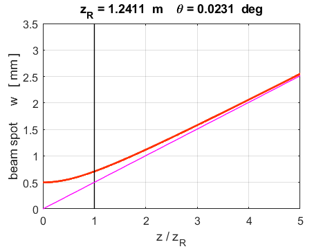
along the axis, the beam spot (9)
Fig. 2. Beam spot w as a function of position z. When z
= 0, we have It is important
to note that the Raleigh range is an indicator of the divergence of the beam.
When When (10) where (11)
Note: the
smaller the value of The shape of a
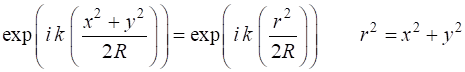
Gaussian beam of a given wavelength Radius of curvature of the wavefront (12) The phase term in equation (7) gives the
curvature of the wavefront which is spherical with radius
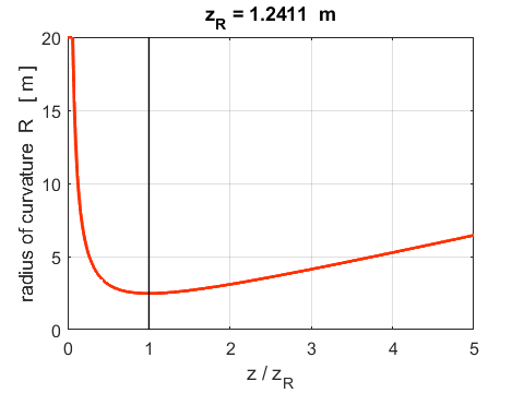
Fig.3. Radius of curvature of the wavefront as a function of z. When z
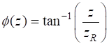
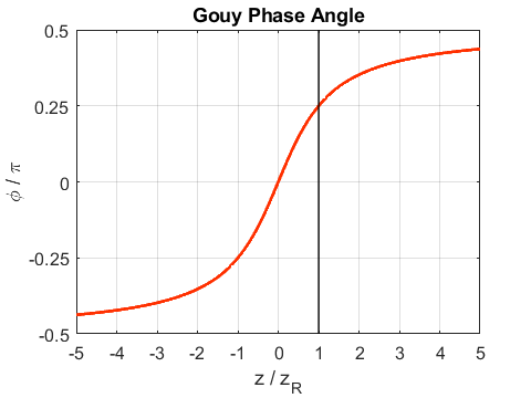
= 0 we have When When Gouy phase (13) The Gouy phase slightly shifts the phase of the wavefront of the wave as a whole. For a focused beam, the dependence of the Gouy phase as a function of z is displayed in figure 4.
Fig.4. Goy phase plot for a focused Gaussian beam. As The most rapid change in phase occurs in the
region from ENERGY: Irradiance
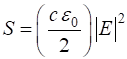
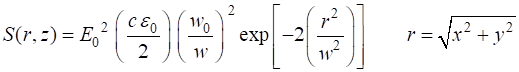
(Intensity) S(r, z) and power P(z) The irradiance (intensity) S is the time average flow of energy per unit time per unit area [W.m-2]. The irradiance S can be calculated from the electric field E of the wave from equation 14
(14) The symbol S is used for the irradiance in the Script and notes and not the
more commonly used letter I. c is
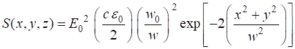
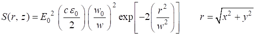
the speed of light and For our propagating Gaussian beam, the electric field E is given by equation 7, so the irradiance S is
(15A) or
(15B)
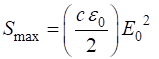
(9) The maximum irradiance occurs at the
location
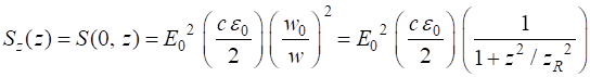
(15C) The variation of the intensity along the
Z axis
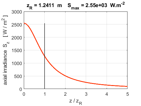
(15D) Figure 5 shows a plot of the axial irradiance Sz as a function of z.
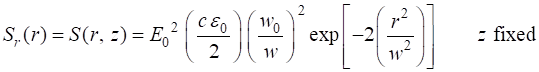
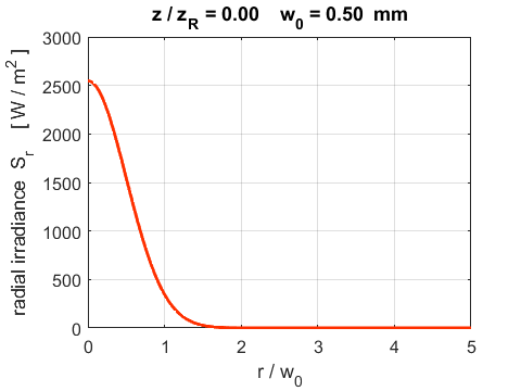
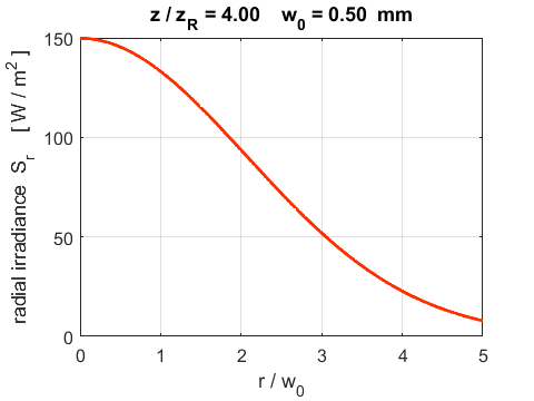
Fig. 5. Axial irradiance When The radial irradiance Sr is the variation in the irradiance in the XY plane located at position z. and typical plots are shown in figure 6.
(15E)
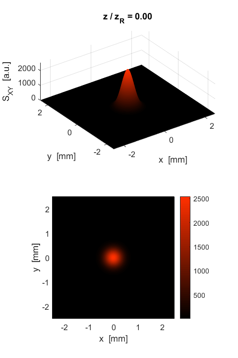
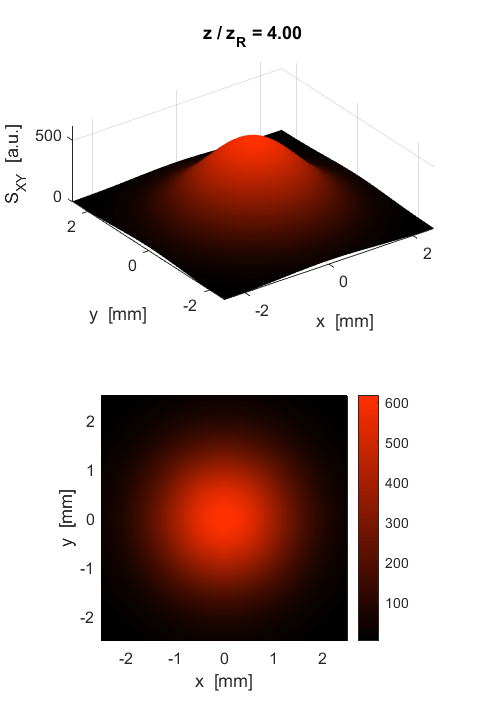
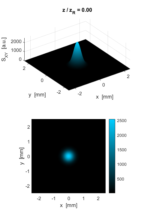
Fig. 6. The variation in the radial irradiance S at two z positions along the axis. The profile of the plots are also a Gaussian function as is the amplitude of the wave. Figure 7 shows the radial irradiance Sr as a [3D] plot and as image that may be viewed on a screen for the same two z positions as in figure 6.
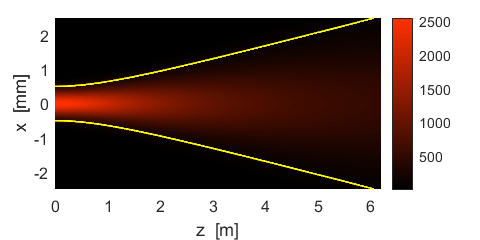
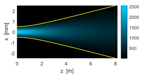
Fig. 7. Beam profile: Radial irradiance Sr. Figure 8 shows the beam in the XZ plane and how the beam diverges and how its intensity decreases with increasing z distance from the waist at z = 0.
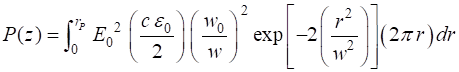
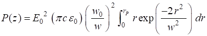
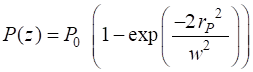
Fig. 8. Profile of the beam in the XZ plane. The yellow lines show the beam spot as shown in figure 2. The power P transmitted through a circular disk of radius rP in an XY plane at position zP is
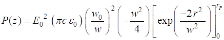
(16A) When
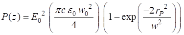
(16B)
If we know the total power
(17A)
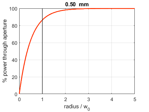
(17B) Figure 9 shows the percentage power that would pass through a circular aperture of varying radius placed perpendicular to the beam at the beam waist.
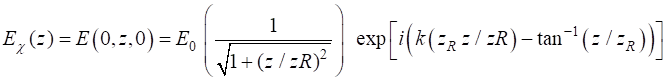
Fig. 9. The percentage power that would pass through a circular aperture of varying radius placed perpendicular to the beam at the beam waist. 86% of the light passes through the aperture when the radius of the aperture is equal to the beam waist. Phase of the wave We can examine the change of phase of the wave along the time Z
axis from equation 7 when (7)
(18) The phase of the wave can be found using the Matlab command angle % phase of the wave along the Z
axis E_chi = E0 .* (1./sqrt(1+z_zR.^2)) .* exp(1i*(k.*zR.*z_zR - atan(z_zR))); chi = angle(E_chi); The
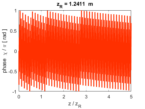
phase along the Z axis is displayed in figure 10.
Fig.10. Phase in the electric
field along the Z axis of the beam. ??? not sure if the graph is correct – get very rapid changes ???
You can easily change any of the
parameters and immediately see the resulting changes. For example: wavelength
for blue light
Fig. 11. Beam profile plots for
blue light
|


|
Ian Cooper email: ian.cooper@sydney.edu.au School of Physics, University of Sydney, Australia http://www.physics.usyd.edu.au/teach_res/mp/mphome.htm |