|
DOING
PHYSICS WITH MATLAB COUPLED
OSCILLATORS PART 1: SINGLE OSCILLATOR MATLAB SCRIPTS oscC001.m Script to model the motion of a single oscillator connected between two springs. Calls the function simpson1d.m (need to download this file). Links VIEW Part 2: Double-oscillator VIEW Part 3: N coupled oscillators – Wave motion on a [1D] monoatomic lattice VIEW Part 4: N coupled oscillators - Wave Motion on a [1D] diatomic lattice INTRODUCTION We can simulate a linear chain of coupled oscillators and emphasize the
properties of the chain which are applicable to mechanical vibrations and
wave phenomena. We will consider a one-dimensional chain of N
particles each of mass mc (c
= 1, 2, 3, … , N). The particles are coupled by massless
springs each with force constant ks
(s = 1, 2, 3, …
, N-1). We let ec
be the
displacement from the equilibrium position of the cth particle along the X axis. The
equilibrium separation distance between particles is a.
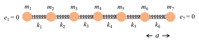
The ends of the
left- and right-hand springs are assumed fixed. Figure 1 shows the
configuration for 7 particles.
Fig. 1
Longitudinal oscillations of 7 particles connected by massless
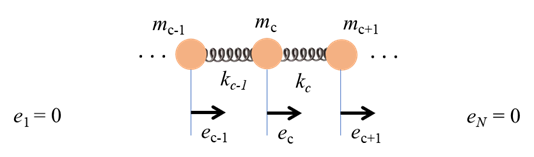
springs. The end particles are always in their equilibrium positions. The elastic restoring force due to
the springs acting on an individual particle is determined by the extension
or compression of the adjacent springs only as shown in figure 2.
Fig. 2. The
elastic restoring force We will assume that a damping force
proportional to the velocity (b damping constant) and a driving
force Fc also act upon each particle. So, the equations of the motion
for the cth particle is given by
(1A) (1B) The left- and right-hand ends of the springs are always assumed to be fixed such that
We can investigate many important aspects of vibrating objects using the Script oscC001.m for the [1D] motion a single particle oscillating between two springs: ·
Simple
harmonic motion ·
Damped
harmonic motion ·
Forced
harmonic motion ·
Natural
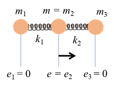
frequency of vibration and resonance Consider the oscillation of a single particle only as shown in figure 3.
Fig. 3. The oscillation of a single particle. The equation of motion for the single particle is then
(4) We approximate the velocity and acceleration using a finite difference scheme
(5)
We can use equation 4 and equations 5 to calculate the displacement from equilibrium at each successive time step. The code to calculate the particle displacement from equilibrium at time step nt+2 is for nt = 1 : Nt-2 e(1,nt+2) = 2*e(1,nt+1) -
e(1,nt) ...
-(k(1)*dt^2/m(1)) * e(1,nt+1) ...
-(k(2)*dt^2/m(1)) * e(1,nt+1) ...
-(dt*b/m(1) )* (e(1,nt+1) - e(1,nt)) ... +
(dt^2/m(1)) * F(1,nt+1); end The displacement is given by the array e(row,column) where the row number gives the particle and
the column is for the time step. The displacement at time step nt+2 depends
on the displacement at the two previous time steps. Therefore, to start the calculations, it is
necessary to specify the displacement and velocity of the particle at the
first two-time steps. For
example, the particle starts with a displacement of 2 mm and zero velocity e(2,1) = 0.002; e(2,2) = 0.002; For a non-zero interval velocity, the input is such that e(2,1) From the calculation of the displacement as a function of time, the
velocity is computed using the Matlab command gradient % Velocity [m/s] v = zeros(1,Nt); v(1,:) =
gradient(e(1,:),dt); and the acceleration is computed form the equation of motion % Acceleration
[m/s^2] a =
zeros(1,Nt); a(1,:) = ( -k(1)*e(1,:) -
k(2)*e(1,:) - b*v(1,:) + F(1,:) ) ./ m(1); All the variables are changed within
the Script. Some of the input variable that you can change include: mass,
spring constant, time steps, time span, damping constant, driving force. The results of the modelling are
displayed in Figure Windows: time evolution graphs for position of particle,
velocity, acceleration; phase plot; animation of motion and one-side power
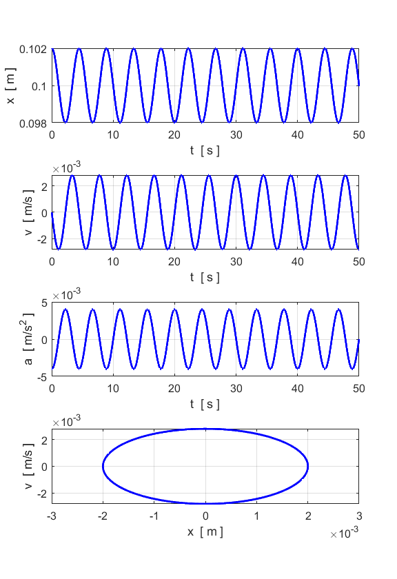
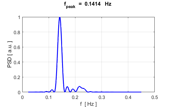
density. The component frequencies of the oscillations for the particle
displacement, can be found from its Fourier Transform by direct integration
(not a fast Fourier Transform) % Fourier Transform
fMin = 0.1*f0;
fMax= 2*f0;
Nf = 201;
H = zeros(1,Nf);
f = linspace(fMin,fMax,Nf);
for c = 1:Nf g = e(1,:)
.* exp(1i*2*pi*f(c)*t); H(c) = simpson1d(g,tMin,tMax);
end
PSD = 2.*conj(H).*H;
PSD = PSD./max(PSD);
[xx, yy] = findpeaks(PSD,f,'MinPeakProminence',0.5);
f_peak = yy;
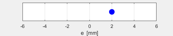
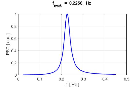
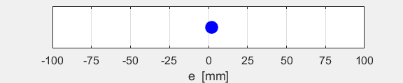
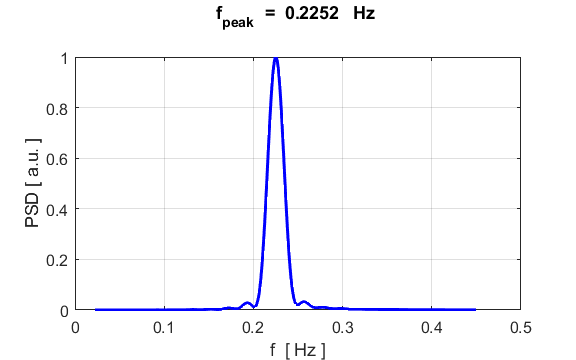
SHM Motion Simulation m = 1 kg k = 1 N.m-1 b = 0 F = 0 e(1) = 0.002 m v(1) = 0 m.s-1
How well do our numerical simulation values compare with the
analytical values? For SHM, a summary of the analytical (A) values and numerical (N)
values are displayed in the Command Window Natural frequency f_A = 0.2251
Hz f_N = 0.2256 Hz Natural period
T_A =
4.4429 s T_N =
4.4318 s Max displacement from equilibrium e_max = 0.0020
m Max velocity
v_A = 0.0028
m/s v_N = 0.0028
m/s Max acceleration
a_A = 0.0040
m/s^2 a_N = 0.0040
m/s^2 There is an excellent agreement
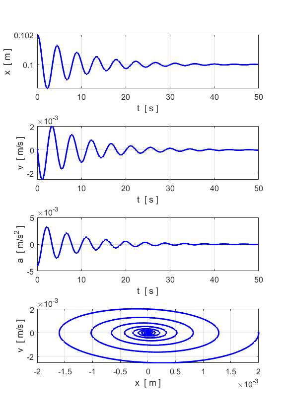
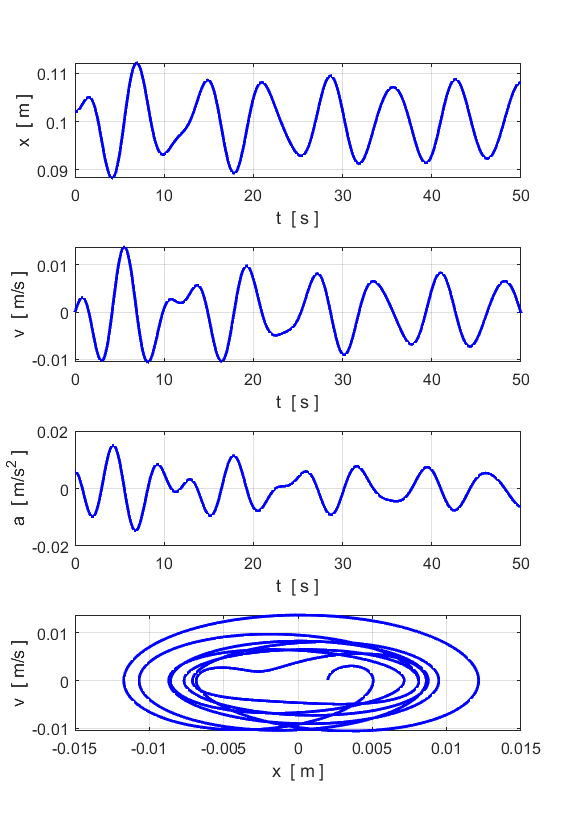
between the analytical and numerical values. DAMPED MOTION You can change the damping parameter
to study the damping of the single oscillator. The following results are for
b = 0.2 and F = 0.
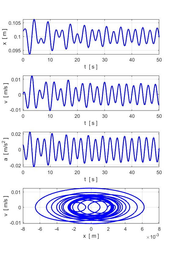
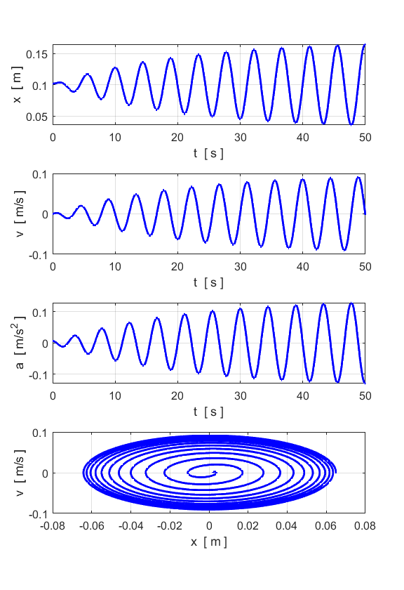
FORCED MOTION and
RESONANCE We can apply a sinusoidal driving
force to the particle and study its response
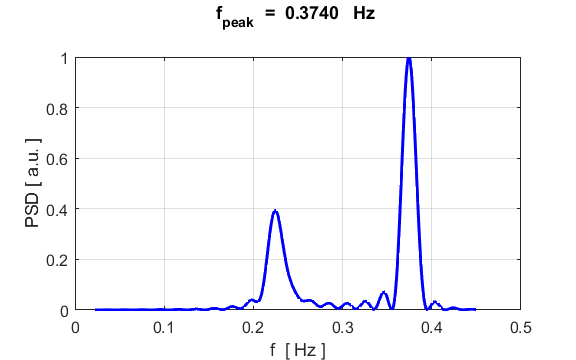
sinusoidal driving force System driven at a frequency greater than the natural frequency
Note the two peaks: one at the
natural frequency and the other much stronger peak at the driving frequency. System driven at a frequency less than the natural frequency
Note the two peaks: the small peak
at the natural frequency and the much larger peak at the driving frequency. System driven at a frequency equal to the natural frequency:
RESONANCE
You get a maximum displacement from the
equilibrium position when the spring is driven at its natural frequency of
vibration. For the case of small damping, the oscillations continue to grow
in strength.
|