|
DOING
PHYSICS WITH MATLAB COUPLED
OSCILLATORS PART 2: TWO COUPLED OSCILLATORS MATLAB SCRIPTS oscC002.m Script to model the motion of a pair of coupled oscillators connected
between three springs. Calls the function simpson1d.m (need to download this file). All the variables are changed within the Script. Some of the
input variable that you can change include: mass, spring constant, time
steps, time span, damping constant, driving force. The results of the
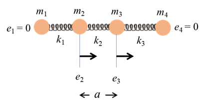
modelling are displayed in Figure Windows and in the Command Window. INTRODUCTION We will consider a one-dimensional chain of 4 particles
each of mass mc (c = 1,
2, 3, 4). The particles are coupled by massless
springs each with force constant ks
(s = 1, 2, 3). Let ec
be the
displacement from the equilibrium position of the cth particle along the X axis. The
equilibrium separation distance between particles is a.
The ends of the
left- and right-hand springs are assumed fixed
Fig. 1
Longitudinal oscillations of 2 particles connected by massless
springs. The end particles are always in their equilibrium positions. We can investigate many important aspects of vibrating systems for the [1D] motion two particles oscillating between three springs using the Script oscC002.m ·
Harmonic
motion ·
Damped
harmonic motion ·
Forced
harmonic motion ·
Modes
of Vibration ·
Natural
frequency of vibration and resonance ·
Fourier
Transform The elastic restoring force (1) We will assume that a damping force (2) where We approximate the velocity and acceleration using a finite difference scheme
(3)
We can use equation 2 and equations 3 to calculate the displacement e
from equilibrium at each successive time step The code used for the implementation of the finite difference method is KS = dt^2.*k; Kb =
b*dt;
KD = dt^2; for nt = 1 : Nt-2 for c = 2 :
N-1 e(c,nt+2) = 2*e(c,nt+1) - e(c,nt)...
-(KS(c-1)/m(c)) *
(e(c,nt+1) - e(c-1,nt+1)) ...
-(KS(c)/m(c)) *
(e(c,nt+1) - e(c+1,nt+1)) ...
- (Kb/m(c))
* (e(c,nt+1) - e(c,nt)) ...
+ (KD/m(c))
* FD(c,nt+1); end end The displacement at time step nt+2 depends on the displacement at the
two previous time steps. Therefore, to
start the calculations, it is necessary to specify the displacement and
velocity of the particles at the first two-time steps. For example, particle 2 starts with a
displacement of 5 mm and zero velocity e(2,1) =
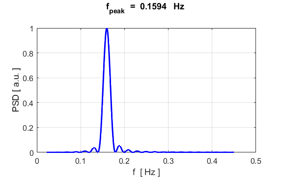
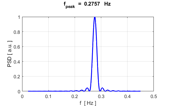
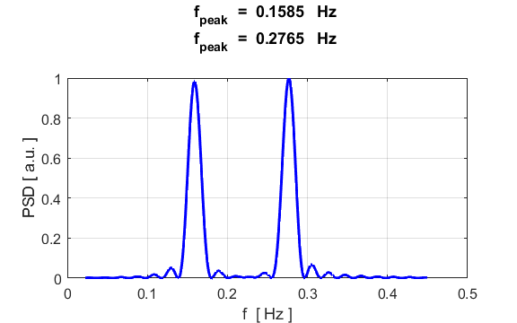
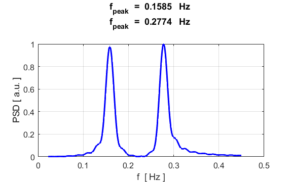
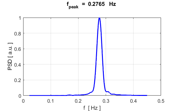
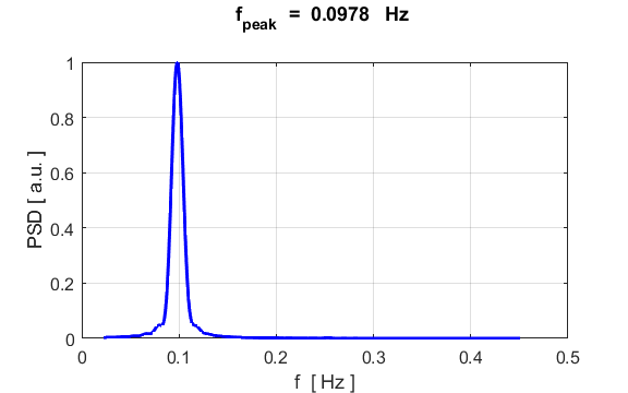
0.005; e(2,2) = 0.005; For a non-zero initial velocity for particle 2, the input is such that e(2,1) The component frequencies of the displacement from equilibrium for
particle 2, can be found from its
Fourier
Transform by direct
integration (not a fast Fourier Transform) % Fourier Transform
fMin = 0.1*f0;
fMax= 2*f0;
Nf = 201;
H = zeros(1,Nf);
f = linspace(fMin,fMax,Nf);
for c = 1:Nf g = e(2,:)
.* exp(1i*2*pi*f(c)*t); H(c) = simpson1d(g,tMin,tMax);
end
PSD = 2.*conj(H).*H;
PSD = PSD./max(PSD);
[xx, yy] = findpeaks(PSD,f,'MinPeakProminence',0.5);
f_peak = yy;
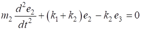
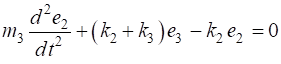
FREE VIBRATIONS: NATURAL MODES For the free motion of the system, the equations of motion for the two
particles are
(4A)
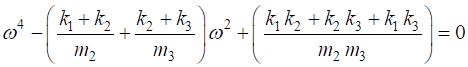
(4B) Assume that the two particles vibrate harmonically with the same
angular frequency
(5)
After much algebra, equations 5 gives a solution to the equation of motions (equations 4), provided
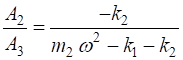
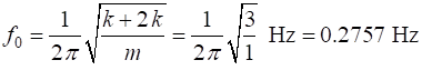
(6) and the amplitudes are given by the ratio (7) Equation 6 is known as the frequency equation and leads to two values for How well do our numerical simulation values compare with the
analytical values? For free motion of the two particles, a summary of the analytical (A)
values and numerical (N) values are displayed in the Command Window. For
example: % Initial conditions [0.0025 m] e(2,1) = 0.005; e(2,2) = 0.005; e(3,1) = 0; e(3,2) = 0; FREE MOTION: Natural modes of vibration Analytical A f_A = 0.1592
Hz f_A = 0.2757
Hz Numerical N (Fourier
Transform peaks) f_N = 0.1585
Hz f_N =
0.2765 Hz There is an excellent agreement
between the analytical and numerical values. The default values for each mass and
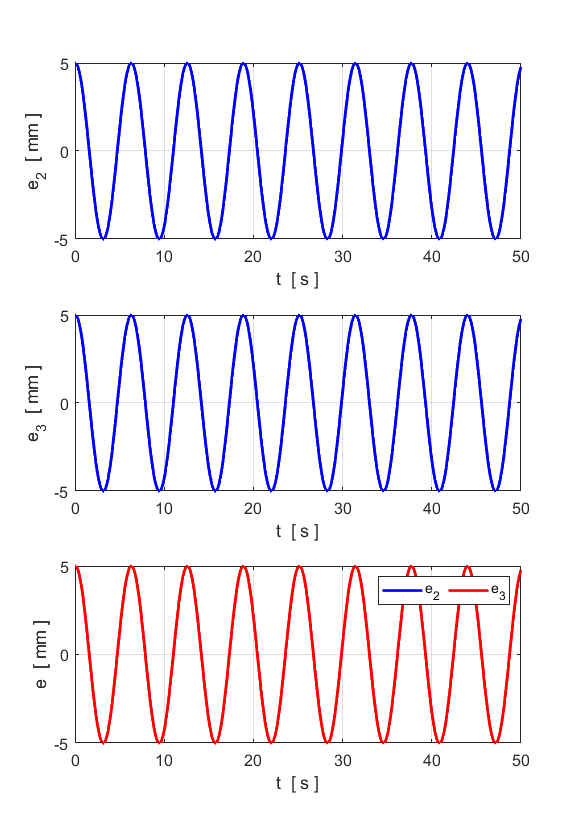
each spring constant are: Simulation #1 SHM % Initial conditions [0.0025 m] e(2,1) = 0.005; e(2,2) =
0.005; e(3,1) = 0.005; e(3,2) = 0.005; The two particles move in the same
direction through the same displacement. The coupling spring is not
compressed or stretched during the motion. Hence, the motion is purely
sinusoidal with the natural frequency
The motion corresponds to two independent single-degree-of-freedom systems.
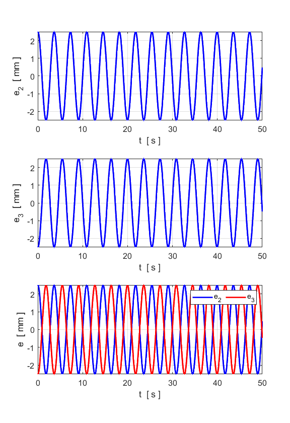
Simulation #2 SHM % Initial conditions [0.0025 m] e(2,1) = 0.0025; e(2,2) = 0.0025; e(3,1) = -0.0025; e(3,2) = -0.0025; The two particles move in opposite
directions but through the same distance. The two motions are
Thus, there are two natural modes of
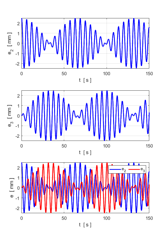
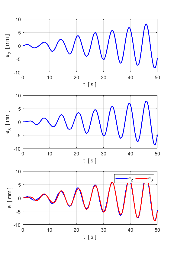
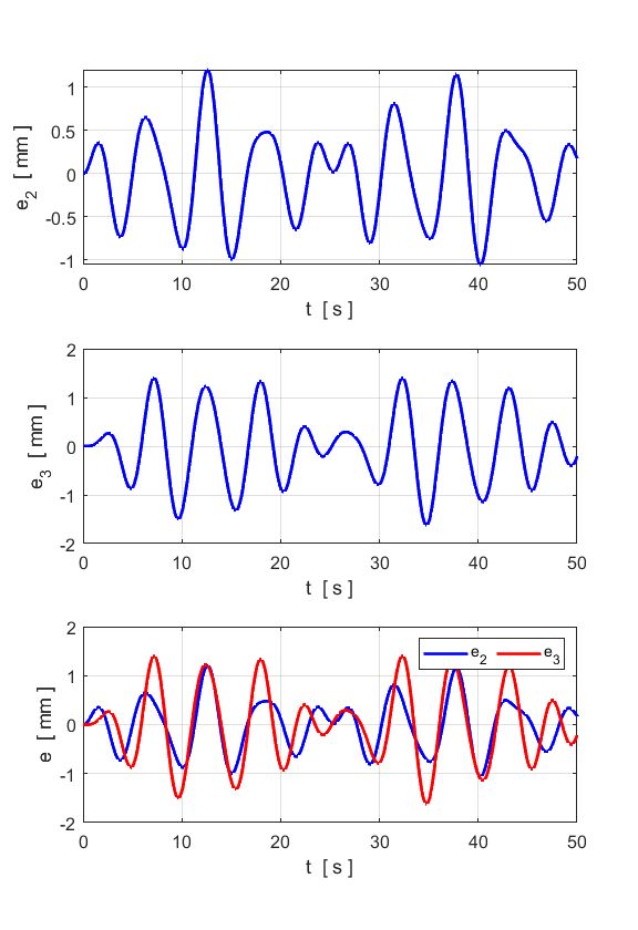
vibration each with its natural frequency as shown in simulations #1 and #2. Simulation #3 Superposition
and Periodic Motion For other initial conditions, the
motion is a superposition of the two sinusoidal natural modes of vibration.
For the initial conditions where the first particle is given a non-zero displacement
while the second particle’s displacement is zero, the first particle
vibrates with large amplitude while the second stands practically still.
After a time, however, the difference in the two frequencies will have
changed the phase between the two vibrations by % Initial conditions [0.0025 m] e(2,1) = 0.005; e(2,2) = 0.005; e(3,1) = 0; e(3,2) = 0;
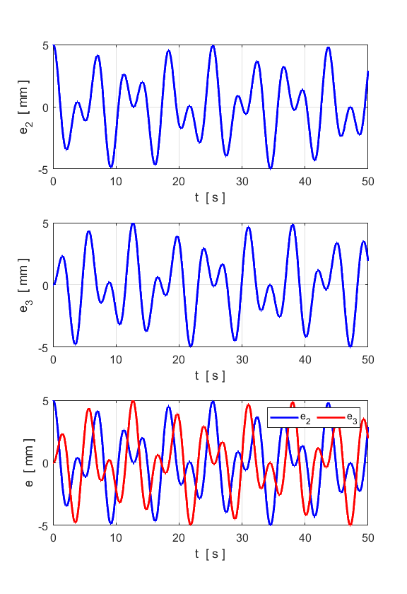
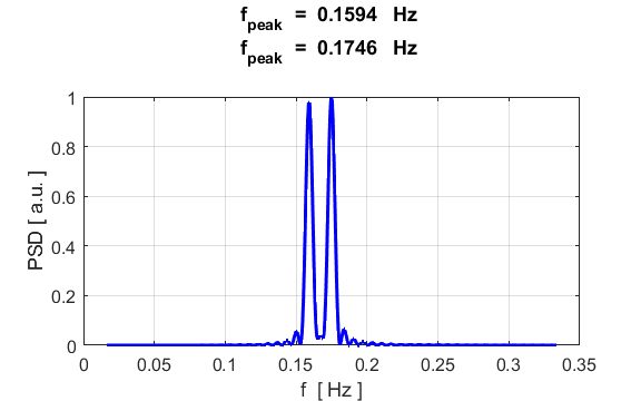
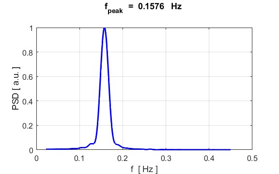
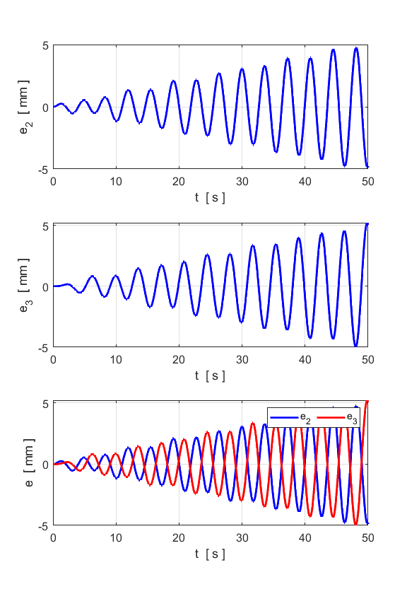
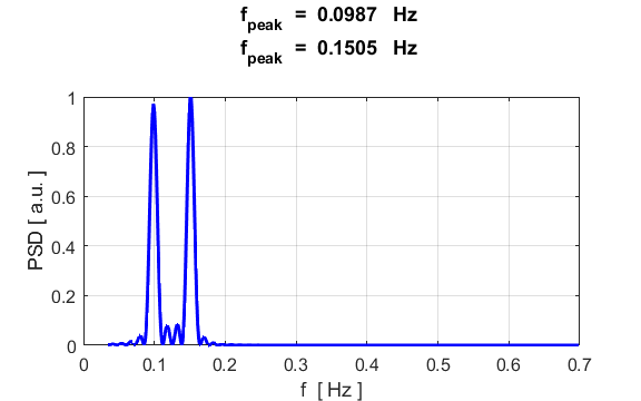
Simulation #4 BEATS When the combined motion of the
particles is not sinusoidal, the motion must be a combination of the two
natural frequencies. When the coupling spring constant k(2) is must less than the spring constants
k(1) and k(3), the two natural frequencies will have values that are close
together and so beats will occur. k(2) =
0.1; % Initial conditions [0.0025 m] e(2,1) = 0.0025; e(2,2) = 0.0025; e(3,1) = 0; e(3,2) = 0;
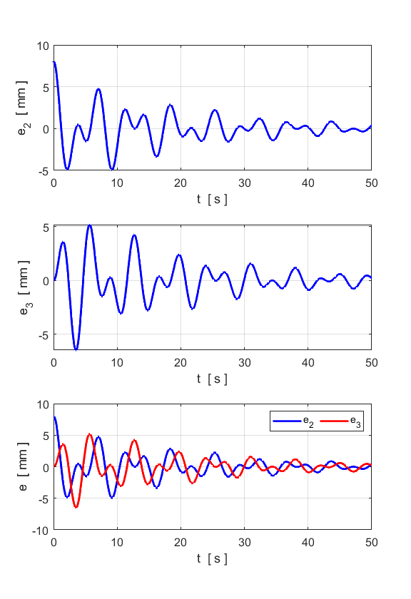
DAMPED MOTION You can change the damping parameter
to study the damping of the coupled oscillators. The following results are
for b = 0.1 and zero
driving force, AD = 0.
Simulation #5 % Initial conditions [0.0025 m] e(2,1) = 0.008; e(2,2) = 0.008; e(3,1) = 0; e(3,2) = 0;
The damping causes the oscillations
to die away. The larger the damping constant b, then the more rapid the decay
in the oscillations. FORCED MOTION and
RESONANCE The default values for each mass and
each spring constant are: We will assume that both particles
start at rest and that the system is not damped (b = 0). % Initial conditions [0.0025 m] e(2,1) = 0; e(2,2) = 0; e(3,1) = 0; e(3,2) = 0; There are two normal modes of
vibration: (1) the particles move in the same direction through the same
distance at a frequency of 0.1592 Hz and (2) the particles move in opposite
directions through the same distance at a frequency of 0.2757 Hz. We can apply a sinusoidal driving
force to particle 2 and study its response of the system to a
sinusoidal driving force % Driving force [N]/Amplitude [0.1
N]/period [1.6T0]/particle number [2] fD0 = 0.2757; AD = 0.0007; FD = zeros(N,Nt); FD(2,:) = AD*cos(2*pi*FD0*t); You can adjust the frequency of the driving force FDO and its
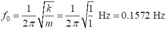
amplitude AD. Simulation #6 Driving frequency
equals normal mode 1 frequency 0.1572 Hz
Simulation #7
Driving frequency equals normal mode 2 frequency 0.2757 Hz
Simulation #8 Driving
frequency not equal to a natural frequency of the system
When the system is driven at one of
its natural frequency, the response is that large amplitudes of oscillation
occur. This phenomenon is called resonance.
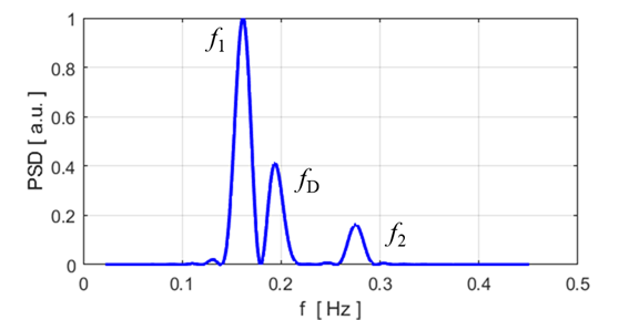
In this simulation, when the system is driven at a frequency that is not
equal to a natural frequency, then the three dominate peaks in the frequency
spectrum where close to the natural frequencies and the driving frequency. Simulation #9 The undamped dynamic
vibration absorber A machine or machine part on which a
steady alternating force of constant frequency is acting may take up
obnoxious vibrations, especially when the driving frequency is close to
resonance. On many occasions, it is not practical or even possible to
eliminate the driving force to reduce the unwanted vibrations. You may
consider changing the mass or spring constant to get way from resonance, but
in many cases, this also is impractical. A third possibility is in the
application of a dynamic vibration absorber. Let the machine part be represented
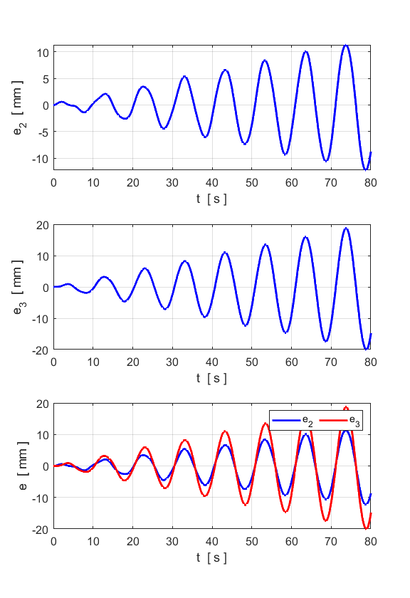
by particle 2 ( Consider the system with the
following specifications: e(2,1) = 0; e(2,2) = 0; e(3,1) = 0; e(3,2) = 0; m(2) = 1; m(3) = 1; k(1) = 1; k(2) = 1; k(3) = 0; AD = 0.0007; fDO =
0.0984;
For our machine part, the oscillations
continue to grow in time and the displacement from equilibrium becomes
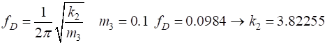
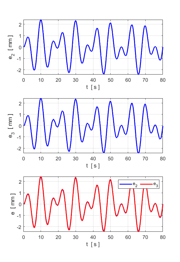
greater than 10 mm. We can set the mass of the absorber
to be
We get an important result. The
oscillations do not continue to grow but reach a maximum steady-state value
of around 2.5 mm. By better selection of the values for |