|
DOING
PHYSICS WITH MATLAB COUPLED
OSCILLATORS PART 3: N-COUPLED OSCILLATORS
Wave Motion on a [1D] Atomic Lattice
MATLAB SCRIPTS oscC00NB.m Plots of the dispersion relationships for a monatomic linear lattice as a function of the propagation constant for the angular velocity, phase velocity and group velocity. oscC00NC.m You can use the Script to explore the propagation along a [1D] atomic lattice for two sinusoidal wave trains and the superimposed wave train. The displacements of the atoms are calculated from analytical expressions. All parameters are changed with the Script. The animation can be saved as an animated gif file.
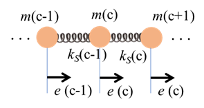
oscC00ND.m A [1D] atomic lattice of N atoms is exciting by driving the displacement of atom 1 by either a single sinusoidal signal or the superposition of two sinusoidal signals. The equation of motions for the atoms are solved using a finite difference method to find the displacement of each atom as a function of time. You can investigate the frequency, phase velocity and group velocity as functions of the propagation constants as the signal propagates through the dispersive medium. All parameters are changed with the Script. The animation can be saved as an animated gif file. oscC00NE.m Explore the natural frequencies of vibration of an atomic lattice of N atoms long a [1D] chain. The system is excited by an external driving force that acts on an atom (an atom located at the location of an antinode is best). The equation of motions for the atoms are solved using a finite difference method to find the displacement of each atom as a function of time. The animation can be saved as an animated gif file. You will need to download the Script simpson1d.m. This Script is used to evaluate a [1D] integral to calculate the Fourier Transform of a signal. The input array to the function must have an odd number of elements INTRODUCTION We will investigate the longitudinal vibrational motion of a [1D] chain of N atoms which are bound to one another by linear elastic forces (figure 1).
Fig. 1. Geometry of the linear lattice.
The equilibrium separation distance between atoms is d. The
mass of the cth
atom is It is assumed that the forces between neighbouring atoms are
Hooke’s law forces, as if the atoms were bound together by massless
ideal springs. At equilibrium, the atoms are situated on equally spaced sites
with a separation distance d. When the chain of
atoms is disturbed, the atoms may execute periodic motion about their
equilibrium positions. The displacement of the cth
atom from its equilibrium position at time t is
given by the displacmenet The elastic restoring force (1) We will assume also that a damping
force (2) We approximate the velocity and acceleration of atom c using a finite difference scheme
(3)
We can use equation 2 and equations 3 to calculate the displacement e
from equilibrium at each successive time step The code used for the implementation of the finite difference method is KS = dt^2.*k; Kb =
b*dt;
KD = dt^2; for nt = 1 : Nt-2 for c = 2 :
N-1 e(c,nt+2) = 2*e(c,nt+1) - e(c,nt)...
-(KS(c-1)/m(c)) * (e(c,nt+1) - e(c-1,nt+1)) ...
-(KS(c)/m(c)) *
(e(c,nt+1) - e(c+1,nt+1)) ...
- (Kb/m(c))
* (e(c,nt+1) - e(c,nt)) ...
+ (KD/m(c))
* FD(c,nt+1); end end The displacement at time step nt+2 depends on the displacement at the
two previous time steps. Therefore, to
start the calculations, it is necessary to specify the displacement and
velocity of the atoms at the first two-time steps. For example, atom 2 starts with a
displacement of 5 and zero velocity e(2,1) =
0.005; e(2,2) = 0.005; For a non-zero initial velocity for particle 2, the input is such that e(2,1) Arbitrary units are used for all quantities or you could use S.I.
units. For many of the simulations, for the motion along our chain of atoms,
we can ignore the terms for the damping force and the driving force. An easy
way to apply the driving force is simply to specify the displacements of
individual atoms at each time step as shown in the code below, where atom 1
is driven by the superposition of two sinusoidal signals. for nt = 1 : Nt-2 for c = 2 : N-1 e(1,nt+1) =
A1*sin(w1*(nt+1)*dt) + A2*sin(w2 *(nt+1)*dt) ; e(c,nt+2) = 2*e(c,nt+1) - e(c,nt)...
-KS * (e(c,nt+1) - e(c-1,nt+1)) ...
-KS * (e(c,nt+1) - e(c+1,nt+1));
end end The component frequencies of the displacement from equilibrium for
particle nE, can be found from its Fourier Transform by direct
integration (not a fast Fourier Transform)
A wave propagates along the chain of atoms. We can estimate its
wavelength by calculating the Fourier Transform of the displacements of all
the atoms at a specified time step. Hence, the estimates of frequency and wavelength means that we can
calculate the phase velocity of a sinusoidal wave along the lattice % FOURIER TRANSFORMS
================================================== % Frequency estimates fPeaks1 and
fPeaks2
fMin = 0.01;
fMax = 5;
Nf = 2901;
H1 = zeros(1,Nf); H2 = H1;
f = linspace(fMin,fMax,Nf);
nE = ceil(N/2);
for c = 1:Nf g = e(11,:)
.* exp(1i*2*pi*f(c)*t); H1(c) =
simpson1d(g,0,tMax);
end
for c = 1:Nf g = e(41,:)
.* exp(1i*2*pi*f(c)*t); H2(c) =
simpson1d(g,0,tMax);
end
PSD1 = 2.*conj(H1).*H1;
PSD1 = PSD1./max(PSD1);
[~, yy] = findpeaks(PSD1,f,'MinPeakProminence',0.6);
fPeaks1 = yy;
PSD2 = 2.*conj(H2).*H2;
PSD2 = PSD2./max(PSD2);
[~, yy] = findpeaks(PSD2,f,'MinPeakProminence',0.6);
fPeaks2 = yy;
% Wavelength estimate lambda
clear g
H3 = zeros(1,Nf); lambda = linspace(2,20,Nf);
xf = 0:40;
fn = e(11:51,Nt)';
for c = 1 : Nf g = fn
.* exp(1i*2*pi*xf/lambda(c)); H3(c) = simpson1d(g,0,40);
end
PSD3 = 2.*conj(H3).*H3;
PSD3 = PSD3./max(PSD3);
[~, yy] = findpeaks(PSD3,lambda,'MinPeakProminence',0.6);
wL_Peaks = yy;
% Propagation velocity: frequency
x wavelength
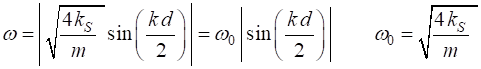
v = wL_Peaks * fPeaks1; FREE MOTION OF THE ATOMS Assuming the only force interactions between
neighboring atoms are the elastic restoring forces, the equation of motion
for the cth atom is (4) We want to find periodic solutions to the equation
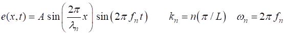
of motion, so we might expect the solution to have the form (5) where Substitution of equation 5 into equation 4 results
in
Hence, (6) The absolute values must
be used, since the frequency is a positive quantity, regardless of whether k
is positive or negative (wave moving to the right or left along
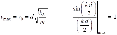
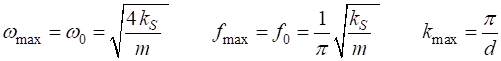
the chain). The maximum angular velocity is Equation 5 gives
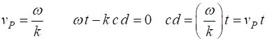
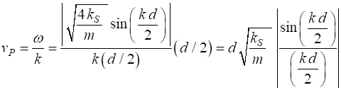
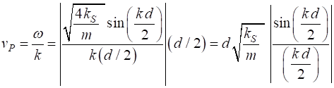
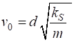
solutions of the equation of motion (equation 4) provided that The phase velocity (7A)
The maximum phase velocity is
(7B)
In general, a wave is a
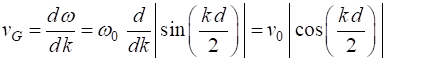
superposition of its harmonic components. The envelope or the group of waves
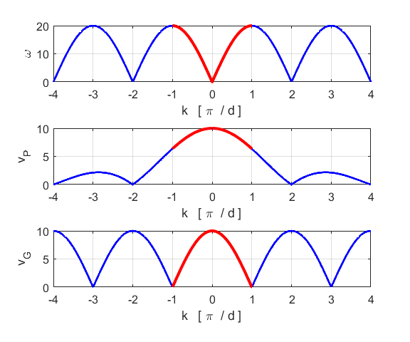
are seen to move forward with a velocity (8) It can be shown that the velocity with which the wave transmits energy along the propagation direction is the group velocity. In a wave train, no energy can ever be transmitted past a node, since the medium at the nodal point is motionless. Thus, the energy must be transmitted with the velocity with which the nodes themselves move, that is, the group velocity. For the case of standing waves, the group velocity is zero, and there is zero net energy flow in this case. The dispersion
relationship (equation 6), the phase velocity
Fig. 2. Dispersion relationships for the monatomic lattice. oscC00NB.m
From the plot of (6) In this long-wavelength
limit, both the phase velocity (9A) (9B) For very long wavelengths, the dispersion effects are negligible and the medium acts like a continuous and homogeneous elastic medium. This is to be expected from a physical point of view, since for such long wavelengths, the atomic nature of the chain is of little importance as far as the dynamics of the system is concerned. As clearly shown in figure 2, as k increases, the dispersion effects become very important. When then the atoms cease to vibrate, and the wave cannot propagate along the lattice. The phase velocity The group velocity This gives the
conditions for standing waves where the phase of the neighbouring atoms differ by Figure 3 to 6 shows the results of running the Script oscC00NB.m or oscC00NC.m with the input parameters: number of atoms N = 21, separation distance between atoms d = 1; mass of each atom m = 0.1, spring constant for each spring kS = 10. (Note: all units are arbitrary)
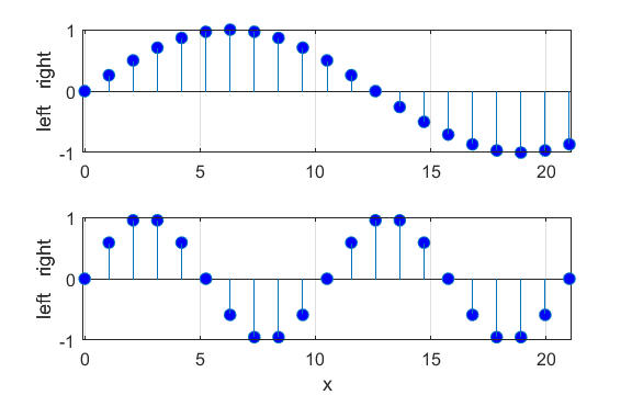
Figure 3 shows the atomic displacements on the monatomic lattice as transverse displacements for convenience of illustration (actual displacements are longitudinal ones in which the atoms are displaced along the chain, rather than normal to it).
Fig. 3. Atomic displacements on the monatomic lattice for a long and short wavelength wave. The displacements are shown as transverse ones for sake of clarity. A positive displacement corresponds to a movement to the right and a negative displacement a movement to the left w.r.t. the equilibrium positions. oscC00NB.m For any given value of k
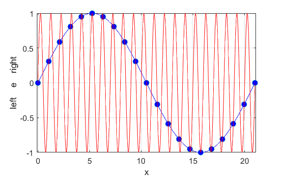
in the region
Fig. 4. A single set of atomic displacements represented by two sinusoidal waves. oscC00NB.m In other words, there
are many representations of the same atomic displacement patterns, each
involving different k values and hence
different difference
Fig. 5. Many values of propagation
constant k
may be associated with any given frequency Thus, any possible
arrangement of atomic positions which is compatible with a sinusoidal
solution of any wavelength, however, short, can be presented as or reduced
(translation by integer multiples of A pure sinusoidal signal
can not transmit information. A sinusoidal wave propagates at a velocity
equal to its phase velocity (equation 9A). So, we will now consider what happens
when two wave trains of the same amplitude A
, one of frequency (10A)
(10B) If we assume The small wavelength
wave propagates with phase velocity (11) The phase velocity of
the envelope corresponds to the group velocity (10)
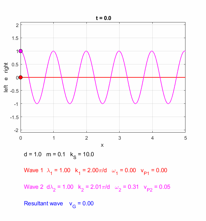
You can use the Script oscC00NC.m to explore the propagation along the [1D] atomic lattice of the two sinusoidal wave trains and superimposed wave train.
If k <<
Fig. 6. In the long wavelength limit, the effects of the dispersion are small, and the two wave trains propagate at approximately the same speeds. The two wave trains have slightly different frequencies and the phase between the two waves continually changes so at once instance the two waves interfere constructively and a little later interfere destructively, producing the beat pattern. The beat pattern as shown by the envelope propagates at the group velocity (equation 10) which is approximately equal to the phase velocity of either wave train. The coloured dots help visualize the motion of the wave trains. oscC00NC.m
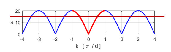
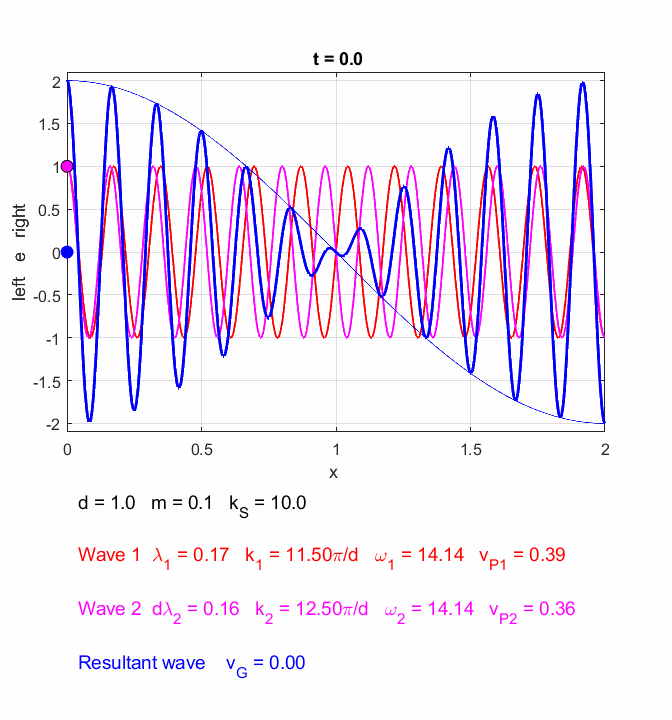
From equation 3 and figure 5, phase
velocity we can conclude that the wave does not propagate as shown in figure 7.
Fig. 7.
Due to dispersion effect, the when a sinusoidal wave has a propagation
constant and wavelength such that An interesting example is shown in figure 8. The two waves have the same angular frequencies but different phase velocities. This results in zero group velocity of the superimposed wave, hence it does not propagate along the atomic lattice.
Fig. 8. The two waves have the same angular frequencies but different phase velocities. This results in a zero group velocity of the superimposed wave. Hence, superimposed wave does not propagate along the atomic lattice. oscC00NC.m The simulation in figure
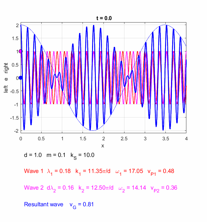
9 gives mysterious results. The envelope propagates at the group velocity
Fig. 9. Due to dispersion effects, the superimposed wave does not propagate along the atomic lattice with a group velocity as predicted by equation 9B. oscC00NC.m But, I am not sure what all the above means!!! Assume that an external force acts on the first atom on the left-hand end of the chain. By disturbing this atom, a wave will propagate along the chain to the right. The frequency of the vibrations will be determined by the external force, and the propagation speed by the elastic and inertial properties of the medium. Thus, the wavelength for the propagating wave and hence the propagation constant are determined by the driving frequency and medium. You cannot specify the propagation constant as indicated in figure 3 to give the frequency of vibration. What do I think the above theory tells us!!! For the input data with the Script oscC00ND.m: number of atoms N = 101, separation distance between atoms d = 1; mass of each atom m = 0.1, spring constant for each spring kS = 10. (Note: all units are arbitrary) The maximum phase
velocity (equation 7) is The maximum frequency (equation 6) for a wave to propagate along the lattice is
You can use the Script oscC00ND.m to investigate the propagation of a wave propagated along the lattice by exciting the motion of atom #1. The default excitation is the superposition of two sinusoidal signals
e(1,nt+1)
= A1*sin(w1*(nt+1)*dt) + A2*sin(w2 *(nt+1)*dt) ; All parameters are changed within the Script. The variables f1 and df
are used as the inputs for the angular frequencies w1 and w2. % INPUT: frequency f = 1 / frequency increment df =
0
f1 = 1;
df = 0; %
INPUT: Amplitude A of waves 1 and 2 A1 =
0.5; A2 = 0.5; %
Angular frequency w (omega) of waves 1 and 2 w1 =
2*pi*f1; f2 = f1
+ df; w2 =
2*pi*f2; Simulation #1 Propagation of a monochromatic wave oscC00ND.m We can model the propagation of the monochromatic
wave through our atomic lattice by driving the displacement of atom #1 by a
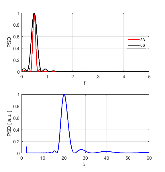
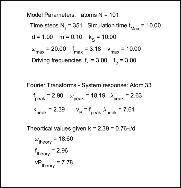
sinusoidal signal of frequency f1. The model parameters are displayed in a
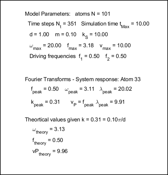
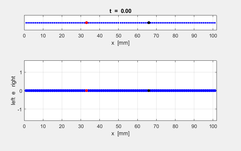
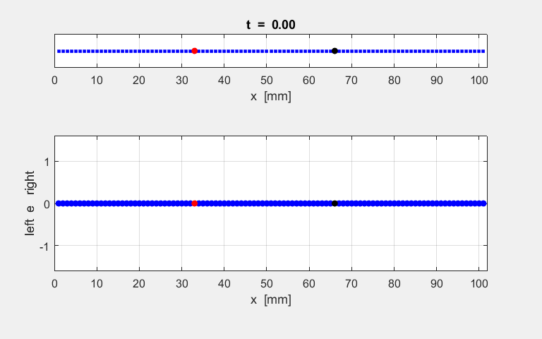
Figure Window as shown in figure S1.
Fig.
S1.1. Table of
model parameters displayed in a Figure Window. The peak value of the
frequency was estimated from the Fourier Transform of the time evolution of
atom #33 and the peak wavelength estimated from the displacement of all the
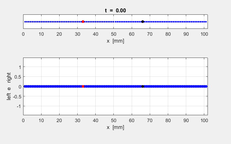
atoms at the end of the simulation time interval. The animated motion of the chain of atoms is shown in figure S2. The
displacements are shown also as a transverse ones
for the sake of clarity in the representation.
Fig. S1.2. Animation
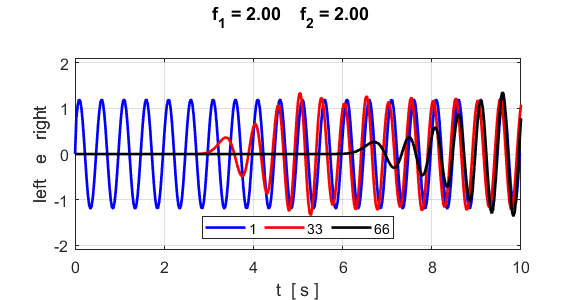
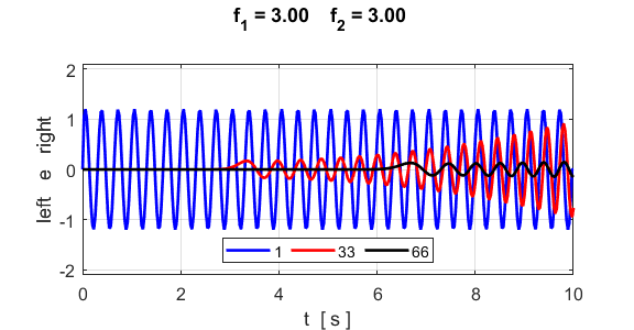
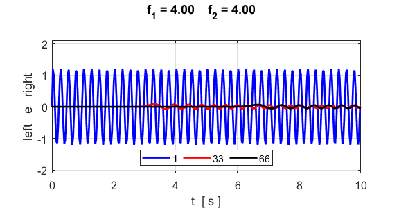
of the motion of a sinusoidal wave propagating along the atomic lattice. The motion of two atoms (#33 and
#66) and the excited atom (#1) as functions of time are
displayed in the following plot. The atoms for the plot are specified by the
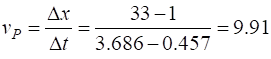
variables n1 and n2. % INPUT: Atoms for Fourier Transform and plots n1 = 33; n2 = 66; The velocity of the peak propagating along the
lattice can be estimated from the plot in figure S1.3 and the estimate agrees
with the value calculated from the Fourier Transforms as shown figure S1.1.
Fig. S1.3 Time evolution of
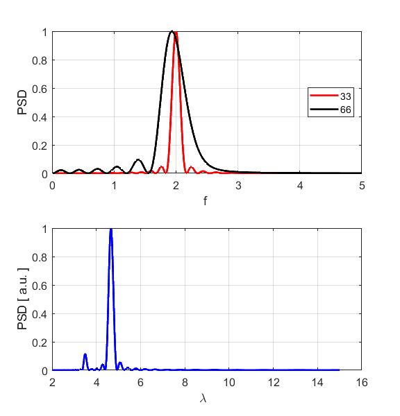
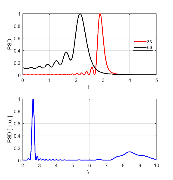
the motion of atoms #1, #33 and #66. By computing
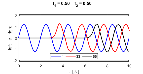
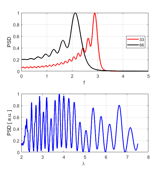
the Fourier Transforms for time/frequency and displacement/wavelength we can
estimate the peak values for the frequency and wavelength respectively and
hence estimate the phase velocity of the sinusoidal wave (figure S1.4).
Fig.
S1.4. Fourier
Transforms showing very distinct peaks.
The results
of the simulation shown that there is a reasonable agreement between the
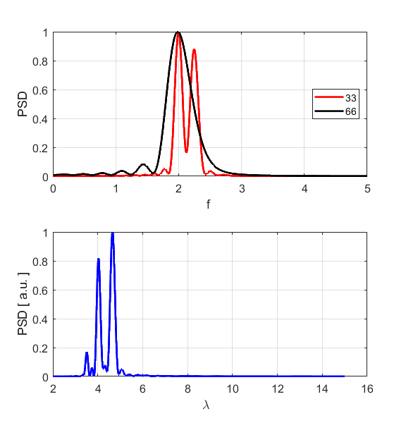
theoretical values for the angular velocity Simulation #2 Propagation of a monochromatic wave oscC00ND.m As you
increase the excitation frequency, the wavelength of the wave decreases
(propagation constant increases) and because of the dispersion effect, the
speed of propagation decreases.
Fig. S2.1.
At the higher frequency of the excitation, the sinusoidal wave
propagates more slowly along the atomic lattice.
Fig. S2.2.
Fig. S2.3. Eventually, each atom will
vibrate at frequency which is close to the driving frequency.
Fig. S2.4. Fourier Transforms. Simulation #3 Propagation of a monochromatic wave oscC00ND.m As the
driving frequency approaches the maximum allowed frequency of vibration, the
speed of propagation falls dramatically. This is shown in the following
simulation when the driving frequency is set to 3.
Fig. S3.1.
The propagation speed is considerably less than the maximum phase
velocity at this high frequency excitation. Again, there is reasonable
agreement between the estimates using the Fourier Transform results and the
theoretical predictions.
Fig. S3.2. At higher frequency the speed of
propagation is less.
Fig. S3.3.
Since the speed of propagation is slower, it takes longer for the wave
to propagate and cause the atoms to vibrate at the excitation frequency.
Fig. S3.4. The Fourier Transforms have
multiple peaks since it takes longer time for a more “pure”
propagating sinusoidal wave to be generated.
Simulation #4 Non-propagating disturbance oscC00ND.m When the driving frequency is set at f1 = 4
which is greater than the maximum allowed frequency (fMax
= 3.18), a propagating wave in not generated, and only a small disturbance
travels along the atomic lattice. This is because the atoms cannot vibrate
with large amplitudes at these high frequencies.
Fig. S4.1. A small disturbance
is propagated along the atomic lattice. and not a sinusoidal wave.
Fig.
S4.2. As shown in the frequency
spectrum, there are no component frequencies with values greater than the
maximum allowed frequency. Since no wave propagates, the wavelength spectrum
is meaningless. Simulation #5 Superposition of two
sinusoidal wave trains oscC00ND.m You can investigate the propagation of a wave
which is the superpositions of two sinusoidal signals. As an example,
consider two waves with frequencies values of 2.00 and 2.25 and amplitudes of
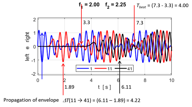
0.60 propagating along a lattice of 101 atoms (m = 0.10 and kS = 10). Propagation of wave #1: frequency = 2.00 wavelength =
4.66
propagation speed = 9.31 Propagation of wave #2: frequency = 2.25 wavelength =
4.03
propagation speed = 9.06 Due to the dispersion, the higher frequency
wave propagates more slowly.
Fig.
S5.1. The two waves
interfere with each other. As the wave propagates, the phase between the two
waves continually changes because of the small difference in frequencies and
the difference in propagation velocities of the two waves. When the waves are
in phase constructive interference occurs and the waves reinforce each other.
At other times the two waves interfere destructively and cancel each other.
The resulting waveform shows the familiar beat pattern.
Fig. S5.2. The two peaks
correspond to the two sinusoidal waves exciting the lattice to vibrate. Wave
#1: From
the displacement from for atoms #1, #33 and #66 you can estimate the beat
period, beat frequency
Fig.
S5.3. Time evolution of the
motion of atoms #1, #11 and #41. From the displacement vs time plot, the beat
period and beat frequency are
which agrees with the theoretical
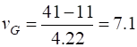
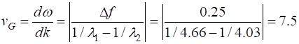
values The estimate for the group velocity is from
the plot is
The estimate of the theoretical group
velocity (equation 7) is
Our two estimates are similar. The envelope
propagates along the lattice more slowly than either sinusoidal wave. NORMAL MODES You can explore the normal modes of vibration that
satisfy the boundary conditions that the displacement at the two ends of the
lattice chain are zero. A normal mode is characterized by a set of stationary
positions for the nodes and antinodes along the chain of atoms. The
longitudinal displacements of the atoms are significant only when the when an
external driving force has a frequency near one of the natural frequencies of
the atomic lattice. This excitation of the system at one of its natural
frequencies is called resonance. The boundary conditions are such that there
are nodes at each end of the chain of N atoms. The equilibrium separation distance between the atoms is d. Hence, the length L of the
lattice is (11) where (12) satisfies the boundary conditions and hence gives a normal mode of vibration of the system. The phase velocity (4A) In the long wavelength regime, k is small, and the phase velocity is essentially constant and equal in value to its maximum value (4B) The maximum frequency and propagation constant of the wave that can propagate along the lattice is (3) But, since there are N atoms in a chain of length L, each
separated by a distance d and the
shortest wavelength
However, the mode Simulation #7 oscC00NE.m The Script oscC00NE.m can be used to explore the behaviour
of the [1D]
atomic lattice. The default input values used in the
simulation are:
Note: if Nt is too small the displacements diverge to infinity. The calculated wave parameters are
Theoretical predictions:
Fundamental mode (1st harmonic)
Harmonic series In running the simulation, it is best to
apply the driving force at the location of an antinode. The driving force is sinusoidal and
specified by its driving frequency fDO,
amplitude AD and the atom being driven nE.
The Fourier Transform (time/frequency) is calculated for atoms n1 and n2. %
>>>>>>>>>>>>>>>>>>>>>>>>>>>>>>>>>>>>>>>>>>>>>>>>>>>>>>>>>>>>>>>>>>>>>
% Driving force parameters: Select an atom at an
antinode for excitation % INPUT: [frequency fD0 = 1/6 Hz /
amplitude frequency AD = 0.08] %
[Particle to be
excited by driving force nE (comment / uncomment)] %
[n1 n2 atoms for Fourier
Transform t/f calculations fD0 = 1/6; AD = 0.08; nE
= ceil(N/2); % odd harmonics % nE =
ceil(N/4); % even
harmonics n1 = nE;
n2 = nE-5; %
>>>>>>>>>>>>>>>>>>>>>>>>>>>>>>>>>>>>>>>>>>>>>>>>>>>>>>>>>>>>>>>>>>>>> The Script is suitable to model only the
longwave harmonics where the velocity of propagation is essentially constant
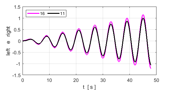
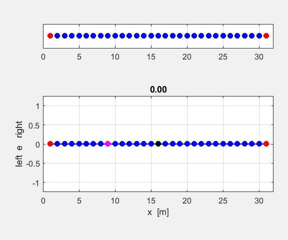
at the maximum value. Fundamental mode n = 1 fD0 = 1/6 AD = 0.08 nE = n1 = 16 n2
= 11
All
atoms vibrate in phase with the same frequency and move in the same direction
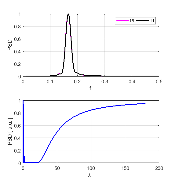
back and forth along the lattice. The peak frequencies are 0.1665 and 0.1666
for atoms 16 and 11 respectively. Theoretical prediction is f1 =
0.1667. The Fourier Transform of displacement could not find the peak
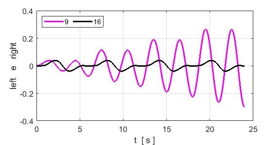
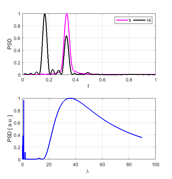
wavelength for the fundamental mode. 2nd harmonic n = 2 fD0 = 2/6 AD = 0.08 nE = n1 = 9 n2
= 16
The
lattice is excited by the driving force applied to an antinode at the site of
atom 9. The 2nd harmonic is excited by the driving force. The
motion of atom 16 corresponds to a node. It is not a “true” node
as this atom vibrates with a small amplitude. The peak frequencies are 0.3329
and 0.3306 for atoms 9 and 16 respectively. Theoretical prediction is f2
= 0.3333. The Fourier Transform of displacement gives a peak wavelength of
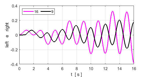
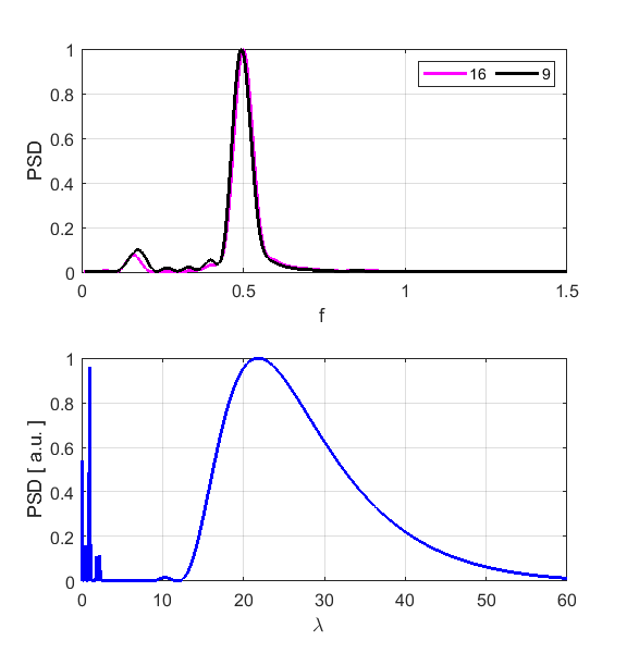
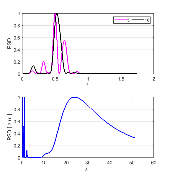
35.8 (theoretical value 3rd harmonic n = 3 fD0 = 3/6 AD = 0.20 nE = n1 = 16 n2
= 9 Note: for higher harmonics, it may be necessary to increase the
amplitude AD of the driving force.
The
lattice is excited by the driving force applied to an antinode at the site of
atom 16. The 3rd harmonic is excited by the driving force. The
motion of atom 16 corresponds to a antinode which
vibrates at the frequency 0.4991 (theoretical prediction is f3 =
0.5000. The Fourier Transform of displacement gives a peak wavelength of 21.8
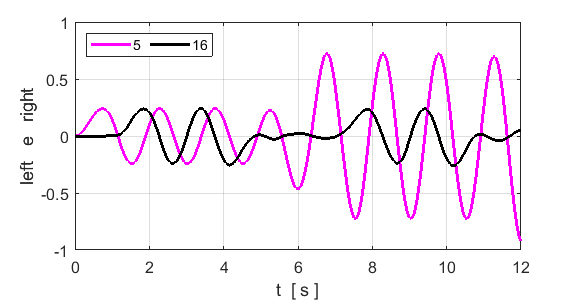
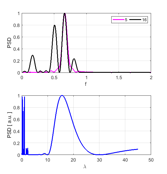
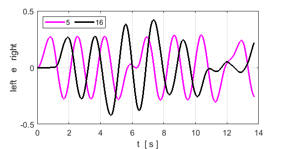
(theoretical value 4th harmonic n = 4 fD0 = 4/6 AD = 1.00 nE = n1 = 5 n2
= 16
The
lattice is excited by the driving force applied to an antinode at the site of
atom 5. The 4th harmonic is excited by the driving force. The
motion of atom 16 corresponds to a node. It is not a “true” node
as this atom vibrates with a small amplitude. The peak frequency at the
antinode site of atom 5 is 0.6653 (theoretical prediction is f4 =
0.6667. The Fourier Transform of displacement gives a peak wavelength of 15.6
(theoretical value Non-resonance excitation fD0 =
3.5/6 AD =
1.00 nE = n1 = 5 n2
= 16 The system
is not driven at one of its natural frequencies of vibration. You get a much
more complicated motion with smaller displacements of the atoms.
System driven at a frequency which is not equal to
one of the natural frequencies of vibration. This results in a more
complicated motion of the atoms and the displacements are smaller than if
driven at a natural frequency. |