DOING PHYSICS WITH MATLAB

COUPLED OSCILLATORS

PART 4: N-COUPLED OSCILLATORS

[1D] DIATOMIC LATTICE

MATLAB SCRIPTS

Matlab Download Directory

oscC00NDE.m

Simulation of the propagation of a disturbance through a diatomic [1D] atomic chain of atoms (atomic lattice). The atomic lattice is excited by a driving force applied to atom #2. A finite difference method is used to calculate the displacement of each atom from its equilibrium position. Plots of the time evolution of three atoms; the spectrums for the frequency and wavelength (Fourier Transforms of displacement with time and position); dispersion relationships for acoustic and optical branches; and a summary of numerical values are displayed in Figure Windows. An animated gif file can be saved to show the motion the chain of atoms in the lattice.

You will need to download the Script simpson1d.m. This Script is used to evaluate a [1D] integral to calculate the Fourier Transform of a signal. The input array to the function must have an odd number of elements

You will need to review Part 1, 2 and 3 for background information and details of the methods used to solve the equations of motion for the longitudinal motion of atoms that form a [1D] atomic lattice.

INTRODUCTION

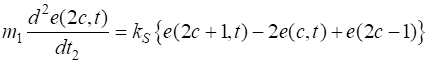
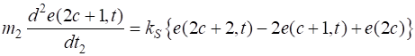
Many common crystals are diatomic compounds, which contain atoms of distinct chemical species. The dynamical characteristics of their lattices differ in several ways from those of monatomic crystals as discussed in Part 3.

Consider a diatomic lattice with the atoms of masses and arranged alternately along the [1D] chain of atoms. The equilibrium separation between atoms is d. The displacement of the c^th atom from equilibrium at time t is . Nearest neigbouring atoms interact with each other via a Hooke’s law elastic restoring forces with spring constant . It is necessary to write two separate equations of motion for each of the atoms with different masses, the result being

(1A)

(1B)

Solutions to the equations of motion (equations 1) are of the form

(2)

provided where is the solution of a quadratic equation which has two solutions, which we will call and as given by equation 3.

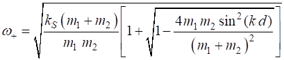
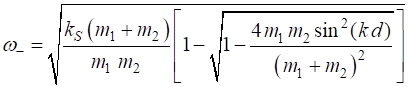
(3A)

(3B)

The solution defines what is called the optical branch and the solution defines the acoustical branch (figure 1). The smallest possible wavelength of the first Brillouin Zone is twice the unit cell distance of the lattice which is .

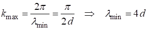
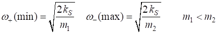
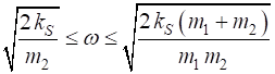
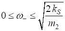
At the boundaries of the first Brillouin Zone

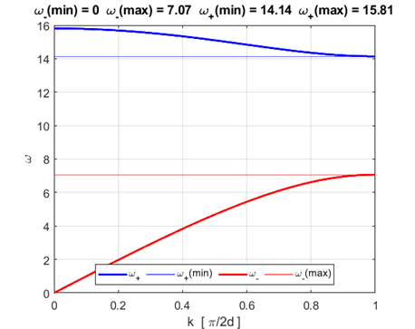
Fig. 1. Dispersion relationship for the diatomic lattice showing acoustical and optical branches and the forbidden frequency band. d = 1 m1 = 0.1 m2 = 0.4 kS = 0

Acoustic branch

In the long wavelength limit:

The two types of atoms move in the same direction with the same amplitude.

Optical branch

In the long wavelength limit:

The two types of atoms move in opposite directions with the smaller mass atoms moving with a larger amplitude, so that the centre of mass of the unit cell remains fixed.

The optical mode of vibrations in ionic crystals, where there are two types of atoms are oppositely charged, can be excited by an electric field, which tends to move the ions in opposite directions. The ionic substance can be excited by the electric field of an electromagnetic wave, hence the term optical is used.

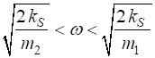
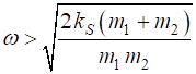
Forbidden frequency region

It is clear from figure 1, there exists a band of frequencies

where there are no solutions of the form given by equation 2. In this frequency range, an undamped continuous harmonic wave cannot propagate along the atomic lattice. If one attempts to excite a frequency in this range, the vibrations are attenuated or damped by the lattice.

For

the lattice simply cannot propagate frequencies in this range, any such disturbances are attenuated or damped by the lattice.

SIMULATIONS

Equation 3 and figure 1 can be misleading. The frequency of vibration is often determined by an external driving force acting on the system and the velocity of propagation of the disturbance depends upon the inertial and elastic properties of the medium. Then, the propagation constant (wavelength) is a function of both the frequency and velocity. In the following simulations a sinusoidal driving force is applied to atom #2 and the respond of the system can be investigated. The frequency f is used rather than the angular frequency . The vibration frequency of two atoms is estimated by calculating the Fourier Transform of their displacements as functions of time and the wavelength of the wave train is estimated by from the Fourier Transform of the displacements of the atoms at the end of the simulation time. From the peaks in the spectrums , the phase velocity is estimated

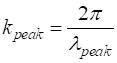
The peak wavelength is used to estimate the propagation constant of the wave

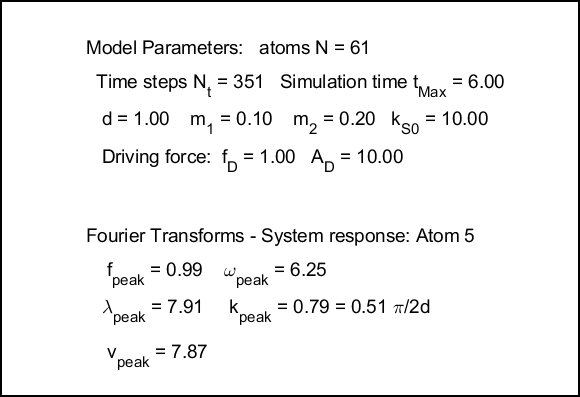
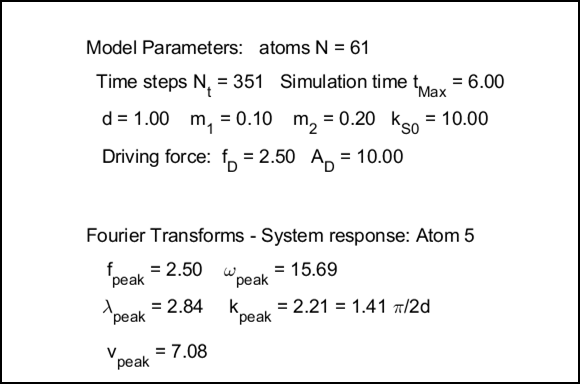
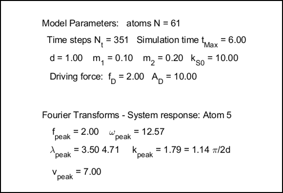
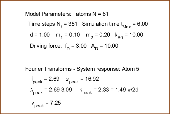
Then we can compare the value of the propagation constant with the value of the propagation constant given by the dispersion relationship (equation 3). At the driving frequency, the value of is estimated from the graph of the dispersion relationship (equation 3).

The default parameters used in the simulations are (arbitrary units):

Number of atoms N = 61

Number of time steps Nt = 351

Simulation time tMax = 6.0

Separation distance between atoms d = 1

Mass of odd numbered atoms m1 = 0.1

Mass of even numbered atoms m2 = 0.2

Spring constant kS = 10

Fourier Transform atoms n1 = 5 n2 = 8

Figure 2 shows the dispersion relationship (equation 3) for the default values.

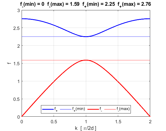
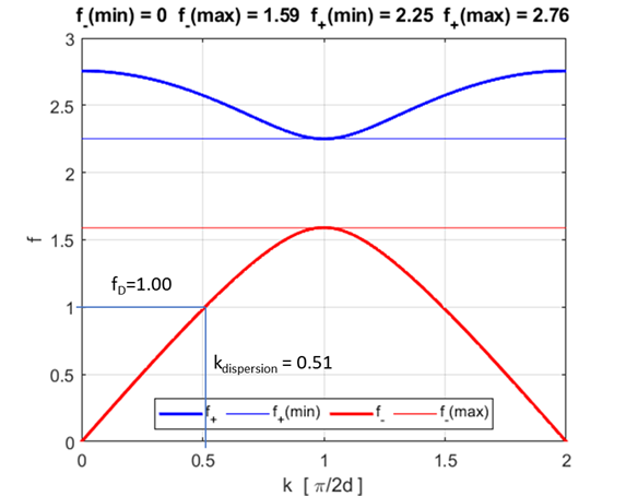
Fig. 2. Dispersion relationship for the diatomic lattice (equation 3). The frequency f is used rather than the angular frequency .

Frequency ranges:

Maximum frequency for propagation of sinusoidal wave through lattice f = 2.76

Optical branch: 2.25 < f < 2.76

Acoustic branch: 0 < f < 1.59

Forbidden frequency band: 1.59 < f < 2.25

Simulation 1 Acoustic branch

Fig. S1.1. Animation of the motion of the atomic lattice.

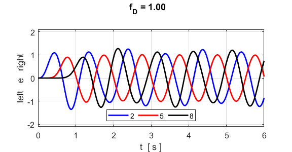
Fig. S1.2. Vibrational motion of atoms 2, 5 and 8.

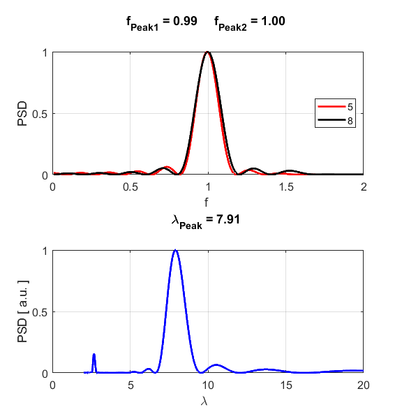
Fig. S1.3. Fourier Transforms are used to calculate the frequency and wavelength of the propagating wave.

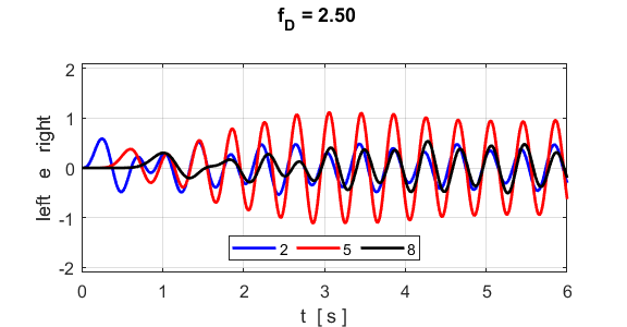
Fig. S1.4. Dispersion relationship. At the driving frequency of fD = 1.00, the propagation constant is k_dispersion = 0.51, which agrees with the value estimated from the peaks in the Fourier Transforms, k_peak = 0.51.

Simulation 2 Optical branch

Fig. S2.1. Animation of the motion of the atomic lattice.

Fig. S2.2. Vibrational motion of atoms 2, 5 and 8.

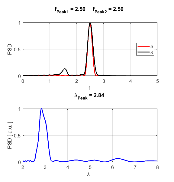
Fig. S1.3. Fourier Transforms are used to calculate the frequency and wavelength of the propagating wave.

Fig. S1.4. Dispersion relationship. At the driving frequency of fD = 2.50, the propagation constant is k_dispersion = 1.40, which agrees with the value estimated from the peaks in the Fourier Transforms, k_peak = 1.41. Note: the value for the propagation constant k_dispersion is in the 2^nd Brillouin Zone and not the 1^st Zone.

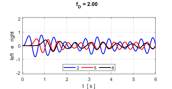
Simulation 3 Forbidden frequency bands

Forbidden frequency band 1.59 < f = 2.00 < 2.76

Fig. S3.1. Animation of the motion of the atomic lattice. A disturbance propagates through the atomic lattice, but after some time the through the vibrations are attenuated.

Fig. S3.2. Vibrational motion of atoms 1, 5 and 8.

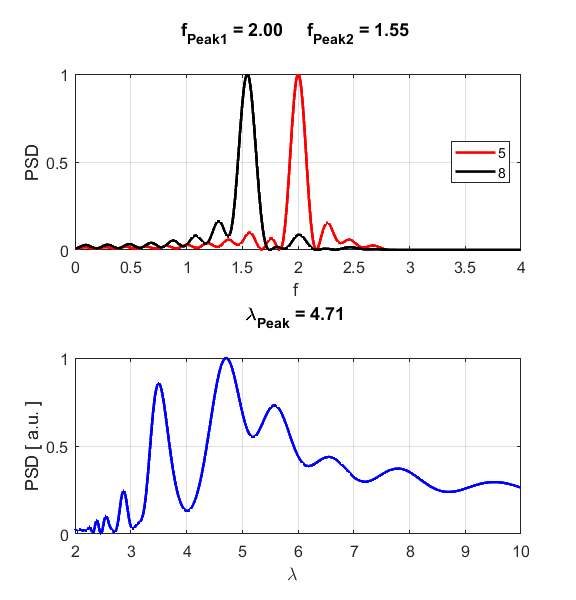
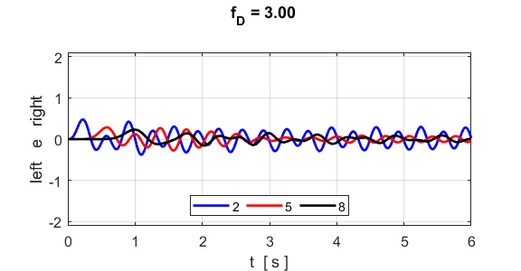
Fig. S3.3. The atoms #5 and # 8 do not vibrate at the same frequency. The wavelength spectrum shows no well-defined isolated peaks, indicating that a sinusoidal wave does not propagate along the lattice.

Forbidden frequency band f = 3.00 > 2.76

Fig. S3.4. Animation of the motion of the atomic lattice. A disturbance propagates through the atomic lattice, but after some time the through the vibrations are attenuated.

Fig. S3.5. Vibrational motion of atoms 1, 5 and 8.

Fig. S3.6. The atoms #5 and # 8 do not vibrate at the same frequency. The wavelength spectrum shows no well-defined isolated peaks, indicating that a sinusoidal wave does not propagate along the lattice.