DOING PHYSICS WITH MATLAB OSCILLATIONS   FORCE VIBRATIONS OF A STRING      RESONANCE Ian Cooper School of Physics, University of Sydney ian.cooper@sydney.edu.au DOWNLOAD DIRECTORY FOR MATLAB SCRIPTS osc_string_drivem.m mscript for the simulation of the forced vibrations of a string fixed at both ends. The driving force produced by an external vibrator is sinusoidal and the frequency of the driving force is entered through the Command Window. The vibrations of the string are animated in a Figure Window. The animated gifs ag_osc_string_driven_**** .gif can be downloaded from http://www.physics.usyd.edu.au/teach_res/mp/images/ STANDING WAVES When a taut string fixed at both ends is disturbed, travelling wave propagate until they reach the ends where they are reflected and travel back along the string. Each such reflection gives rise to waves travelling in opposite directions. The waves along the string interfere with each other according to the principle of superposition. 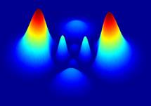Standing waves can be setup along the string where all points execute simple harmonic motion with the same phase and frequency. 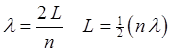A standing wave is described by      (1)          for a string of length L, to satisfy the boundary conditions at x = 0, y = 0 and x = L, y = 0, the propagation k must have a set of discrete values      (2)         Hence, the allowed wavelengths of the string are      (3)         For a standing wave, multiples of  must fit into the length L. Fixed points that have the largest displacement along the string are called antinodes and points which have the zero amplitude are called nodes. The antinodes are spaced at intervals  apart and so the nodes are also spaced at  intervals. 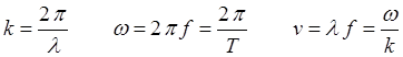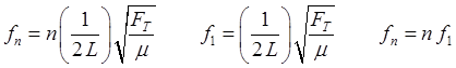The speed of propagation v of the wave along the string depends upon the string tension FT and linear density      (4)          Using equations (1), (2) and (3) it is clear that the frequencies for the vibration the standing waves in the string form a harmonic series where f1 is called the fundamental or the 1^st harmonic      (5)          and fn is the n^th harmonic. The harmonics are referred to as the natural frequencies of vibration of the system. RESONANCE In general, whenever a system capable of oscillating is acted upon by a series of impulses having frequency equal to nearly equal to one of the natural frequencies of oscillation of the system, then, the system can oscillate with relatively large amplitude. This phenomenon is called resonance and the system is said to resonate. In the Matlab simulations using the mscript  osc_string_drivem.m  we will consider a guitar string with parameters:        length  L = 0.80 m     string tension  FT = 400 N     = 4.00x10^-4  kg.m^-1 (parameters can be changed in mscript) The natural frequencies of the string from equation (5) are      625 Hz,   1250 Hz,   1875 Hz ,   2500 Hz , 3125 Hz, … The mscript osc_string_drivem.m  solves the one-dimensional wave equation using a finite difference method . The boundary conditions are a node at one end of the string x = L, y = 0 and an applied sinusoidal driving force of frequency fD at the other end x = 0      The value for the frequency fD of the driving stimulus is entered in the Command Window and the respond of the string is animated in a Figure Window. The value of the amplitude AD can be changed in the mscript, its default value is chosen to be small so that the end of the string at x = 0 is approximated as a node. 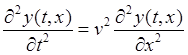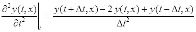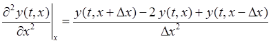THE WAVE EQUATION The one dimensional wave equation can be expressed as      (6)       Using a finite difference method, the second partial derivatives are approximated by      (7)             and         Therefore, the wave equation can be approximated to give an equation to estimate the value of y at time  from the known values of y at times  and      (8)        Matlab code for the driving force for ct = 1:Nt    y(ct,1) = A .* sin(wD .* t(ct));     % time variation of driving force    end Matlab code for solving wave equation y = zeros(Nt,Nx);           % initilize wave function    y(:,end) = 0;               % boundary condition at end of tube    % Solving the Wave equation by FDTD method --------------------------------    for ct = 2 : Nt-1 for cx = 2 : Nx-1           y(ct+1,cx) = 2*y(ct,cx) - y(ct-1,cx) + K * (y(ct,cx+1) - 2* y(ct,cx) + y(ct,cx-1)); end    end SIMULATIONS String driven at its fundamental frequency  f1 = 625  Hz In our model of the vibrating string any dissipative forces are ignored. When the driving force matches any of the natural frequency of vibration of the string, energy is continually being transferred from the driver to the string. As a consequence, the amplitude of the oscillation grows and grows with time. String driven at 500 Hz The driving frequency is not equal to any of the natural frequency of vibration of the string. The string does not resonate – the waves travelling forward and backward along the string do not interfere to produce nodes and antinodes at fixed locations along the string. Energy is not efficiently transferred from the vibrator to the string and energy is also transferred back to the vibrator from the string, so the amplitude of the oscillation remains small. String driven at a frequency equal to the 2^nd harmonic   fD = 2 f1 = 1250  Hz String driven at a frequency equal to the 3^rd harmonic   fD = 3 f1 = 1875  Hz String driven at a frequency equal to the 4^th harmonic   fD = 4 f1 = 2500  Hz String driven at a frequency equal to the 5^th harmonic   fD = 5 f1 = 3125  Hz For a true standing wave the nodes occur at fixed locations along the string and are point where the string is permanently at rest. Hence, energy is not transported along the string to the right or left. The energy remains “standing” in the string as energy is continually being transferred between elastic potential energy and vibrational kinetic energy in the region between the nodes. In our simulation of the string’s vibrations, the end at x = 0 is not a “true” node since this end of the string does not remain permanently at rest. If you carefully observe the animated motion of the string you will also see that there are no “true” nodes. There can’t be true nodes as energy must flow along the string from the stimulus driving the oscillations at the end of the string. Energy is continually added to the string by a vibrator, building up the amplitude of the oscillation only at or near one of the natural frequencies of vibration. When the string is excited at a frequency well away from a natural frequency, the reflected waves reaching the end of the string at x = 0 are out of phase with the external vibrator, hence energy can be transferred from the string back in to the vibrator. The wave pattern is not fixed but wiggles about. On average, the amplitude of the oscillation is small and not much different from that of the vibrator. Hence, the string absorbs maximum energy from the vibrator at resonance. Tuning a radio is an analogous process: the circuit resonates with the transmitted signal and absorbs peak energy from the radio signal.