DOING PHYSICS WITH PYTHON


Ian Cooper

matlabvisualphysics@gmail.com


DYNAMICAL NON-LINEAR SYSTEMS

LOGISTIC DIFFERENCE EQUATION


DOWNLOAD DIRECTORIES FOR PYTHON CODE

       Google drive


       GitHub


pyChaos001.py

The logistic difference equation   for the population  is iterated for the specified initial population  and growth parameters r. The output gives an animated plot of the iterated values of the population  for increasing values of r.


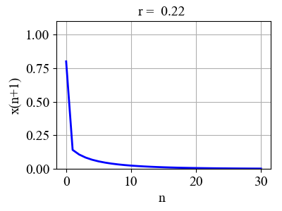
pyChaos002.py

The logistic difference equation  for the population  is iterated for the specified initial population  and growth parameters r.

Plots:  ,   iteration steps ,  Bifurcation diagram, Lyapunov Exponent, time plot (iteration steps)  x(n) vs n.


pyChaos0003.py

Mapping function F for period 4 dynamics

Plot: F vs x    F = x,   |dF/dx|  and equilibrium points

Warning: code not perfect in finding the equilibrium points where F = x. Need to change the number of grid points and the tolerance.


INTRODUCTION

Biologists studying the variability in populations of various species where generations do not overlap found a simple difference equation that predicted the population trajectories reasonably well. One such equation is a simple quadratic equation called the logistic difference equation. Very surprising, this simple difference equation predicts under certain circumstances a fantastically complex and chaotic behaviour that was total unexpected.


The logistic difference equation is given by

(1)              


where x(n) is a scaled population at iteration n and r is the control or growth parameter. The initial condition is specified by  where .  Each iteration can be considered as a single time step. The dynamics of this system is controlled by the single growth parameter r. The dynamical motion of the phenomenon is non-linear because of the quadratic term in the population .


                   This simple non-linear system does not possess simple dynamical properties


It is often observed in nature that a population x will increase from one generation to the next when small and decrease when large. This is expressed mathematically by the product . Figure 1 displays the parabola with growth parameter r  = 0.75 for logistic difference equation (equation 1). If x(n) = 0 or 1 then x(n+1) = 0. The maximum increment  in one iteration occurs when x(n) = 0.5 and x(n+1) = 0.75 = r.

Fig. 1.   Parabolic plot for the logistics
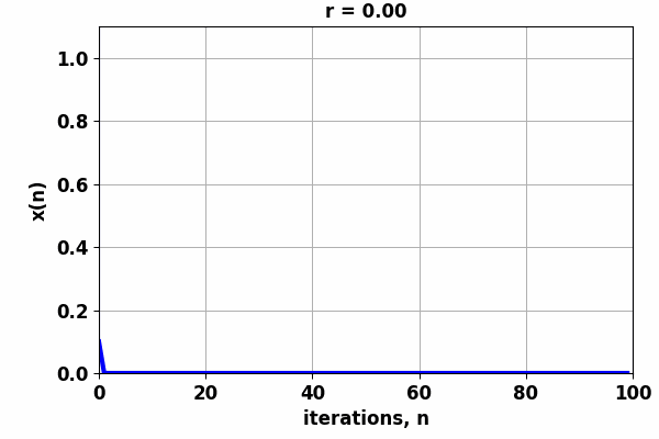
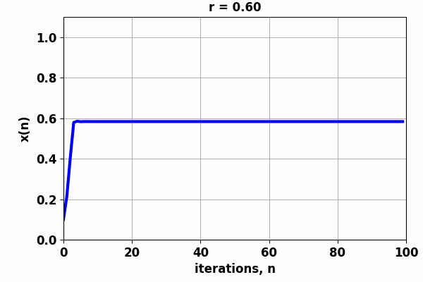
 equation   .

pychaos002.py


The population is computed for many time steps n = 1, 2, 3, . . .  , Nmax.  Nmax is chosen large enough so the initial transient fluctuations in the population can be ignored.


The dynamics of the logistic difference equation is best displayed by observing an animation of the population x(n) as the growth factor r is incremented. For small values of r, the population converges to a stable equilibrium population. However, as the value of r increases, interesting things happen as shown in figures 2 and 3.


Fig. 2.   Population x(n) as the growth factor is incremented from 0 to 1. As r passes through a critical value, complete changes in the dynamics of the system occur.            pyChaos001.py


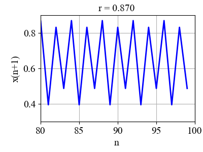
Fig. 3.   Population x(n) as the growth factor is incremented from 0.6 to 1.    pyChaos001.py


When r > ~0.75,  no longer converges to a single equilibrium population, but it oscillates between two values. This characteristic change in behaviour is called a bifurcation. Increasing the growth factor even further results in  oscillating between not two, but four values. This phenomenon is called period doubling.  As one continues to increase the growth parameter then  goes through bifurcations of period eight, then sixteen, . . . , then chaos! When growth parameter r > ~ 0.9, the population  neither converges or oscillates, but its value becomes completely random and the behaviour is largely chaotic. However, there is a particular value of r where the sequence again oscillates and period doubling occurs as r is slightly incremented.


This complicated dynamical behaviour is show in a bifurcation diagram and a plot of the Lyapunov exponent (figure 4).

Fig. 4.   Bifurcation diagram - plot of the iterated values of  as a function of the growth parameter r.  Note the transitions from stable equilibrium populations to oscillation and period doubling to chaotic behaviour and region of periodic behaviour within the region of chaos.  Lyapunov exponent :   is an indicator of chaotic behaviour.     pyChaos002.py


A useful analytical metric that can help characterize chaos is called the Lyapunov exponent, which measures how quickly an infinitesimally small distance between two initially close states grows over time. This is expressed by the equation


where the LHS is the distance between two initially close states after t steps, and the RHS is the assumption that the distance grows exponentially over time.  λ is the Lyapunov exponent which is measured for a long period of time (ideally  ). If  λ > 0 then small distances grow indefinitely over time, which means the stretching mechanism is in effect for chaotic dynamics (the folding mechanism is not captured in this Lyapunov exponent). If λ < 0 then small distances don’t grow indefinitely, i.e., the system settles down into a periodic trajectory eventually. The equation for the Lyapunov exponent can be transformed into a more easily computable form (pyChaos002.py)


Thus, the Lyapunov exponent is a time average of
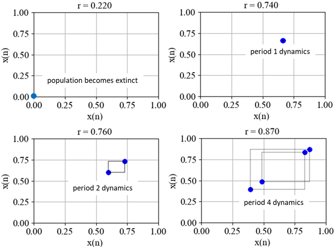
   at every state of the system.


PERIOD 1 DYNAMICS         

The orbit of the population x is attracted to an equilibrium point or fixed point  when , therefore,


Since , the only fixed point for  is  which means that the population will become extinct.  The equilibrium population  is a stable fixed point. A requirement for a non-zero fixed-point  point is that r > 1/4.

Fig. 5.   If   then the population will become extinct   for all initial values of the population x(0).                          pyChaos002.m


We 
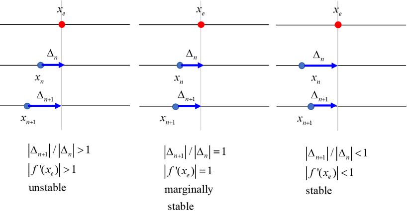
can derive analytical expressions for the fixed points of the [1D] map   to check the stability of the fixed points  and   .


To determine the stability of the fixed points , we let


and we have


If  then the orbit will iterate away from since .


If  then the orbit will iterate towards since .


Thus, the local stability criteria for a fixed point are shown in figure 6.

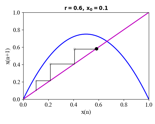
Fig. 6.   Stability of fixed points.


The first derivative for the non-zero equilibrium point   where r < 1/4  is


Thus, for the equilibrium point  to be stable requires


Therefore, we can conclude


The local curvature of the curve  determines the change in x each time f  is iterated. At a fixed point, only when the local slope is less than one, does the next iterated population approaches a stable fixed point, otherwise, the next iterated value of the population diverges from the unstable fixed point. So, for  the dynamics of the orbit is completely known, the population will eventually converge to one of the two fixed points irrespective of the initial population . 


This dynamic is said to be period 1:


Figure 7 shows plot for the case when r = 0.6. This is a stable fixed point since .

Fig. 7.   Plots of the iterated population  when for different initial populations x0 = 0.10 and x0 =0.80. The stable fixed point is  and its value is independent of the initial population and the iteration converges from its initial population to the equilibrium population in a few time steps.     pyChaos002.py


PERIOD DOUBLING DYNAMICS

The bifurcation diagram shown in figure 8 shows an expanded version of the figure 1 plot. It clearly shown the change in the dynamics in the evolution of the population when .

Fig. 8.   Bifurcation diagram - plot of the iterated values of  as a function of the growth parameter r .  Note the transitions from stable equilibrium populations to oscillation and period doubling to chaotic behaviour and region of periodic behaviour within the region of chaos.    pyChaos002.py


When , the fixed points of  f  become unstable and the orbit bifurcates to a cycle of period 2. Now, the population x returns to the same value only after every second iteration, that is


and there are now two attractors of f(x) with fixed points
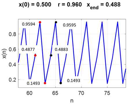
  and .


Fig. 9.   Period 2 dynamics .  The population x oscillates between the two fixed points . Hence the population x only returns to the same value after every second iteration . Note: at each fixed point .     pyChaos002.py

What happens when the value of r is slightly increased slightly above 3/4? We know from our observations the single fixed point becomes unstable and gives birth (bifurcates) to a cycle of period 2. The population x returns to the same value only after every second iteration

the range  ?


The period 2 dynamics is only exhibited in the range
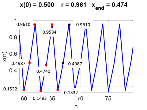
 . If  another bifurcation occurs and the cycle of f  is period 4. The period 4 iteration is


Fig. 10.   Period 4 dynamics .  The population x oscillates between the four fixed points . Hence the population x only returns to the same value after every fourth iteration. At each fixed point .               pyChaos002.py


Figure 11 shows another way in which to analyse the population dynamics for r = 4. The mapping function f4(x) (blue curve); the gradient of the mapping df4/dx (magenta curve); f4 = x (red curve) are plotted against the population x.  The dots show the equilibrium populations xe where the blue and red curves intersect,  . The only stable equilibrium points are those with . The code pychaos003.py used for figure 11 has a problem in finding too many or too few crossing points and it is necessary to adjust the number of grid points and the tolerance (the crossing point at x = 0.713 is not identified).  The crossing points displayed in the Console are:

           xe              |df/dx|

          0.000        1.000            unstable

          0.394        0.343            stable

          0.433        1.000            unstable

          0.486        0.433            stable

          0.832        0.389            stable

          0.856        1.000            unstable

          0.870        0.258            stable


Fig. 11.   Period 4 dynamics .  The population x oscillates between the four fixed points . Hence the population x only returns to the same value after every fourth iteration. At each fixed point .                    pyChaos003.py   


Increasing r again will lead to further bifurcations. This phenomenon is called period-doubling

        period 1 à period 2 à period 4 à period 8 à period 16 à  . . .

 Fig. 11.   Period 8 dynamics .  The population x oscillates between the eight fixed points (x returns to the same value after every eighth iteration.    pyChaos002.py    chaos23.pptx  


Increasing r again , the changes in population x become chaotic where the evolution of the population never repeats itself and if the initial population is slightly changed it can give rise to very different orbits even after a small number of iterations.


Fig. 12.  Population orbits in the chaotic regime . After a small number of iterations, there are two very distinct orbits for the two initial values  (blue) and  (red).      pyChaos0002.py   


Fig. 13.  Bifurcation diagram. Plot of iterated values of x(n) as a function of the growth rate r.      


Fig. 14.   Period 1 orbit in a narrow window within the region of chaos.


Figure 15 shows another animated view of the changing population dynamics for increasing values of the growth parameter r.


Fig. 15.   The population orbit for increasing values of the growth parameter r.  pyChoas001.py
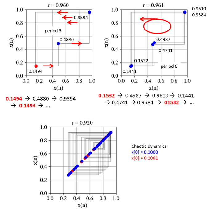


Period doubling window

In the period doubling window, periodic motion again occurs where odd period dynamics may occur as shown in figures 16 and 17.


Fig. 16.   Period 3 dynamics                      


Fig. 17.   Period 6 dynamics produced by the bifurcation of the period 3 dynamics                     


PERIOD DOUBLING – 
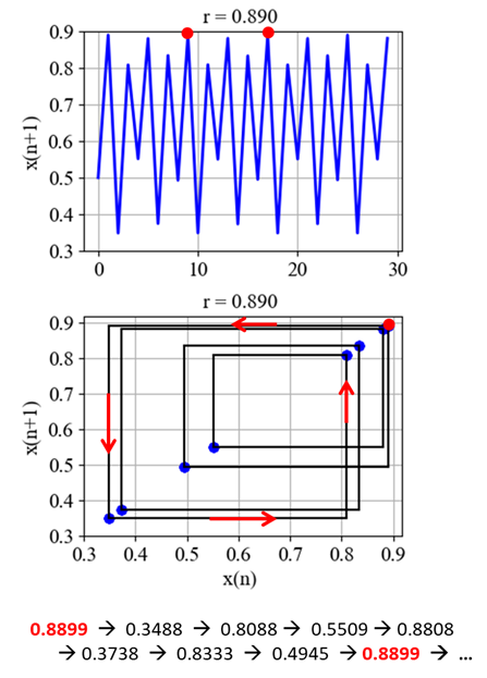
FINDING THE FIXED POINTS OF THE DYNAMICS

We can show the dynamics of the logistic difference equation another way by plotting the points (x(n), x(n)) for increasing values of n after any initial transience no longer influences the dynamics. Figure 18 shows the lot with r = 0.890 for period 8 dynamics and who the population cycles through 8 fixed-points.

Fig. 18.   8 period dynamics.                    pyChaos002.py   chaos23.pptx


Fig. 19.  Period doubling and chaotic dynamics.                             pyChaos002.py   chaos23.pptx


The logistic difference equation is an exceptionally simple model of the population growth for   butterflies who lay eggs their eggs in year n and their offspring are born in year .  If there are zero butterflies  then no butterflies and no eggs, hence . At the other extreme, , then the competition for food is so great that they do not lay eggs, so again .


References

H. Gould & J. Tobochnik   An Introduction to Computer Simulation Methods (Part 1)


R. M. May Simple Mathematical Models with Very Complicated Dynamics, Nature 261, 459 (1979)