Matlab Physics

TIME DEPENDENT QUANTUM MECHANICAL SCATTERING IN TWO DIMENSIONS

Ian Cooper

Any comments, suggestions or corrections, please email me at

matlabvisualphysics@gmail.com

MATLAB

qm2DB.m

A finite difference time development method (FDTD) is used to solve the two dimensional time dependent Schrodinger Equation. This method is applied to the free propagation of a Gaussian pulse and the scattering of the pulse from different potential energy functions: wall, cliff, single slit, double slit and Coulomb (Rutherford scattering). The variable flagU is used to select the potential. The results of the computations are presented as colour graphs portraying the probability density function. The amplitude of the probability for the scattered wave is often very small, so the probability density can be scaled to better display the scattering (scattering factor sF 1). Arbitrary units are used for all quantities. Values of the wavefunction and potential energy are calculated on a [2D] mesh for a square of length 1. The centre of the square has Cartesian coordinates (0.5, 0.5). The initial wavefunction is a plane with a [2D] Gaussian envelope. The wavefunction is zero at the boundaries of the square. So, when the wave packet strikes the boundaries, reflections occur. This results in interference patterns developing because of the superposition of the incident and reflected waves. I do not know how to apply absorbing boundary conditions to eliminate the reflections (someone might be able to help me). The motion of the pulse can be saved as an animated gif file (flagG). For different simulations, you will need to change some of the input parameters.

The animations evolve slowly. Not sure how to speed them up.

math_ft_kx2D.m (Math_ft_kx1.m F.T. Gaussian function)

Fourier transform by direct integration for the [1D] Gaussian wave packet.

simpson1d.m

Function to evaluate an integral using Simpson’s rule. Must use an odd number of grid points.

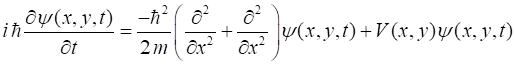
THE 2-DIMENSIONAL SCHRODINGER EQUATION

In the time-dependent approach, the initial state of the system is specified by an initial wavefunction. This wavefunction is then allowed to evolve through time as governed by the kinetic and potential energies of the system. The initial state of the system is described by a Gaussian wave packet which propagates in the +X direction.

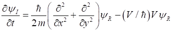
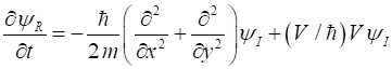
In 2 dimensions and Cartesian coordinates (x, y), the Schrodinger equation can be expressed as

(1)

The wavefunction is a complex function

(2)

where the real part of the wavefunction is and its imaginary part is .

Using equations 1 and 2 and equating the real and imaginary parts, the Schrodinger equation becomes

(3A)

(3B)

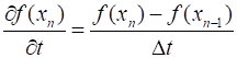
We can use the finite difference time development method to solve the 2D Schrodinger equation. Time and position are defined at a set of discrete points

(4A)

(4B)

(4C)

The finite difference approximation assumes that the derivates of a function can be expanded in a Taylor series around every point of the mesh up to a desired order of accuracy.

The first derivative can be approximated as

(5A) forward difference

(5B) central difference

The second derivative is approximated as

(5C)

The finite difference approximation from equations 1 to 5 at time step for the mesh point becomes

(6A) time steps

(6B) time steps

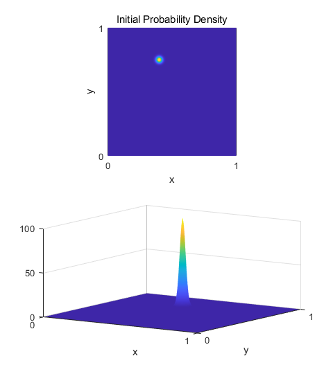
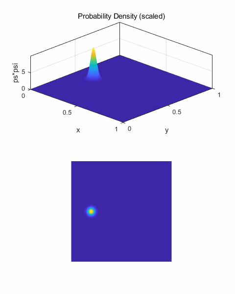
MATLAB qm2DB.m

The Script qm2DB.m uses arbitrary units for all quantities. The initial pulse is a plane wave with a [2D] Gaussian envelope. The number 1 attached to a variable represents the current time and a 2 represents the value of the variable at the next time step.

% [2D] GAUSSIAN PULSE (WAVE PACKET) ==================================

% Initial centre of pulse

x0 = 0.20; y0 = 0.5;

if flagU == 6

x0 = 0.40; y0 = 0.75; % y0 impact parameter

end

% Initial amplitude of pulse

A = 10;

% Pulse width: sigma squared [5e-3]

s = 1e-3;

% Wavenumber [50]

k0 = 20;

% Envelope

psiE = A*exp(-(x-x0).^2/s).*exp(-(y-y0).^2/s);

% Plane wave propagation in +X direction

psiP = exp(1i*k0*x);

% Wavefunction

psi1 = psiE.*psiP;

% Probability Density

prob1 = conj(psi1).*psi1;

% Extract Real and Imaginary parts

R1 = real(psi1); I1 = imag(psi1);

Fig. 1. Initial wave packet (pulse)

The wavefunction is calculated at each successive time step and half time step by calling the functions shown below. The number of time steps is given by the variable nT.

% FUNCTIONS ==========================================================

% psi1 (current value at time t)--> psi2 (next value at time t+dt/2 & t+dt

% functioin pisI at times t+dt/2, t+3dt/2, ....

% function psiR at times t+dt, t+2dt,

function I2 = psiI(N, I1, R1, dt, U, f)

I2 = zeros(N,N);

x = 2:N-1;

y = 2:N-1;

I2(x,y) = I1(x,y) + f*(R1(x+1,y)-2*R1(x,y)+R1(x-1,y)+R1(x,y+1)-2*R1(x,y)+R1(x,y-1))...

- dt*U(x,y).*R1(x,y);

end

function R2 = psiR(N, R1, I1, dt, U, f)

R2 = zeros(N,N);

x = 2:N-1;

y = 2:N-1;

R2(x,y) = R1(x,y) - f*(I1(x+1,y)-2*I1(x,y)+I1(x-1,y)+I1(x,y+1)-2*I1(x,y)+I1(x,y-1))...

+ dt*U(x,y).*I1(x,y);

end

Then the current value of the probability density function is displayed in a Figure Window.

figure(1)

set(gcf,'units','normalized');

set(gcf,'position',[0.05 0.1 0.30 0.70]);

set(gcf,'color','w');

for c = 1:nT

% Update real prt of wavefunction

R2 = psiR(N, R1, I1, dt, U, f);

R1 = R2;

% Update imaginary part of wavefunction

I2 = psiI(N, I1, R2, dt, U, f);

% Probability Density Function

prob2 = R2.^2 + I1.*I2;

I1 = I2;

subplot(2,1,1)

. . .

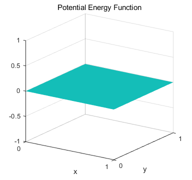
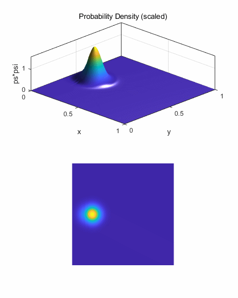
Simulation 1 Free propagation of the wave packet

We can model the free propagation of the wave packet that initially is moving in the X direction. The potential energy function is set to zero at all mesh points.

Fig. 2. Zero potential energy field.

Figure 3 shows an animated view for the motion of the wave packet. The wave number is k0 = 100 and there are 500 time steps. As the wave packet propagates, it spreads in all directions. The spreading is due to the different wavelength components of the wave packet travelling at different speeds. Components with larger wave numbers (smaller wavelengths) corresponds to waves of larger momentum, energy and velocity.

(7)

One can clearly see, the faster components moving head of the wave packet peak in figure 3.

Fig.3. Animated view for the motion of the wave packet in free space.

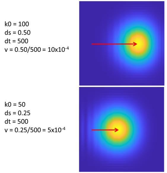
Fig. 4A. The greater the wave number k0, the faster the wave packet propagates in the X direction. For k0 = 100, the peak is displaced by 0.50 units, whereas when k0 = 50, the peak is only displaced by 0.25 units in 500 time steps. The values are in agreement with the predictions of equation 7.

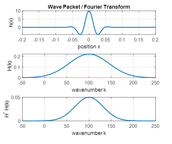
The spreading of wave packets is a subtle example of Heisenberg uncertainty principle and the superposition of states. Since the extent of the wavefunction is restricted, then the uncertainty in momentum must be greater than zero. Therefore, the wavefunction must contain components other than simply and these can combine in such a way that at time t = 0 for the wavefunction to travel only in the +X direction. However, at later times, the components will add so that the wavefunction propagates in the Y direction as well, and thus the wavefunction spreads in all directions as time evolves.

The Script math_ft_kx2D.m can be used to find the Fourier Transform of a [1D] version of the initial Gaussian wave packet (k0 = 100). Figure 4B shows the [1D] Gaussian wave packet and its Fourier Transform. The Fourier Transform is Gaussian in shape with the peak at k = 100 which corresponds to the value of k0.

Fig. 4B. The initial wave packet (k0 = 100) and its Fourier Transform and power density function.

Simulation 2 Wave packet striking a potential wall

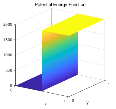
The scattering of the wave packet depends upon the relative values of the packets energy and the height of the potential wall. Figure 5 shows a potential wall with a height of 1000 a.u..

Fig. 5. A potential wall with a height of 2000 a.u.

The energy of the packet can be taken as . When k0 = 50 a.u., E = 2500 a.u. Figure 6 shows the scattering for a potential wall of height 2000 a.u. and figure 7 for a potential wall of height 5000 a.u.

Fig. 6. Scattering of E = 10000 a.u. (k0 = 100) wave packet from a potential wall of height 2000 a.u. The pack packet propagates well past the edge of the wall. Part of the wave is reflected and interferes with the incident wave.

Fig. 7. Scattering of E = 2500 a.u. wave packet from a potential wall of height 2000 a.u. The wave packet barely penetrates pass the edge of the wall. Part of the wave is reflected and interferes with the incident wave. Constructive interference peaks are clearly visible.

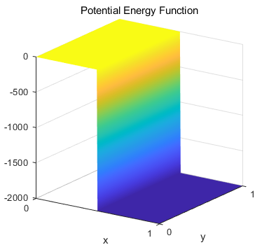
Simulation 3 Wave packet striking a potential cliff

The wave packet is scattered by a potential cliff as shown in figure 8. Figure 9 shows the scattering of the wave packet.

Fig. 8. A potential cliff with a drop of 2000 a.u..

Fig. 9. Scattering of wave packet (k0 = 50) from a potential cliff. The greater the energy of the wave packet, the greater the penetration pass the edge of the cliff.

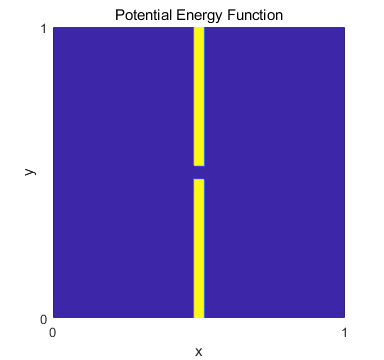
Simulation 4 Wave packet striking a single slit

This is a simulation of the scattering of an electron by a single slit. The wave packet is reflected by the barrier and diffracted at the slit as it passes through the it (figures 10 and 11). The diffracted wavefunction is very small magnitude and so it is necessary to use a small scaling factor sF = 0.1.

Fig. 10. Potential energy function for single slit diffraction

Fig. 11. Single slit diffraction. Wave packet spreads (diffracts) in passing through opening. Most of the wave packet is reflected at the potential barrier and interferes with the incident wave creating an interface pattern.

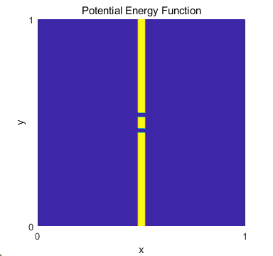
Simulation 5 Wave packet striking a double slit

This is a simulation of the scattering of an electron by a double slit. The wave packet is reflected by the barrier and diffracted at the slit as it passes through the it (figures 12 and 13). The diffracted wavefunction is very small magnitude and so it is necessary to use a small scaling factor sF = 0.1.

Fig. 12. Potential energy function for a double slit.

Fig. 13. Double slit diffraction. Wave packet spreads (diffracts) in passing through opening. A very predominant interference pattern is displayed with very distinct regions of constructive and destructive interference. The wave packet is reflected at the potential barrier and interferes with the incident wave creating an interface pattern.

Simulation 6 Rutherford Scattering from a Coulomb Potential

The FDTD method is applied to the Rutherford scattering in two dimensions. Much of what is known about atoms, nuclei and subatomic particles has been gained from the results of scattering experiments. Usually the experiments involve a localized electron beam of incident particles at the beginning, and a measured distribution of scattered particles, at the end. The [2D] simulations provide a very intuitive picture of what happens in a scattering event. 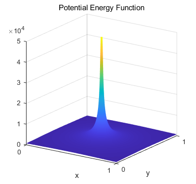We can think of our simulations modelling the scattering of alpha particles from a stationary sample of gold foil. For alpha particle scattering, the dominant interaction between an alpha particle and a stationary gold nucleus is their Coulomb repulsion. The collision process is three-dimensional. However, the two-dimensional modelling conveys the essential features of the processes.

Fig. 14. Potential energy function for Rutherford (Coulomb) scattering.

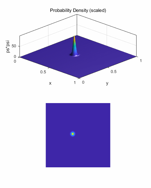
We have seen from the above simulations that the quantum-mechanical wave packets spreads over time, so care much be taken in the starting coordinates of the initial wave packet. The effect of different impact parameters is achieved by placing the initial wave packet at different y coordinates (y0). The results of the computations are shown in the following plots.

Figure 15 shows the results of a “head-on” collision (y0 = 0.5). We see that throughout the collision the wave packet remains symmetric about the Y coordinate y = 0.5, a consequence of the symmetry in a zero impact scattering event. As time proceeds, the wave packet spreads and it becomes distorted in shape forming curved band travelling in the –X direction. The leading edge of the wave packet is reflected from the scattering centre (backscattered) and is interfering with the remainder of the wave packet.

Fig. 15. The time evolution of the probability density for a “head-on” collision. Impact parameter b = 0, y0 = 0.5;

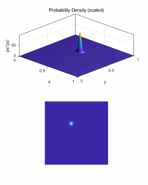
Figure 16 shows the scattering for impact parameter b = 0.02 (y0 = 0.52). The probability density function is asymmetrical. The wave packet is mainly backscattered in the direction 100^o w.r.t. the +X axis.

Fig. 17. The scattering for impact parameter b = 0.06 (y0 = 0.56). The probability density function is asymmetrical. The wave packet appears to be “squeezing” past the scattering centre. The wave packet is strongly distorted by the Coulomb repulsion when it is near the scattering centre, but is relatively free to spread on the side away from the scattering centre. The deflection of the wave packet is about 70^o to the initial incident direction along the X axis.

Fig. 18. Scattering for large impact parameter. The overall distortion of the wave packet in noticeably less than shown in figures 16 and 17, since the wave packet is farther from the scattering centre and hence is less influence by it. The wave packet is more deflected than scattered. The scattering angle has been reduced to about 45^o.

The Script could be modified to stimulate the scattering of 8 MeV alpha particles from a stationary gold nucleus. If you do this modification, please email the Script.