QUANTUM MECHANICS

ELECTRON BEAMS IN FIELD-FREE SPACE

Ian Cooper

matlabvisualphysics@gmail.com

qmElectronBeamA.m

Simulation of an electron matter wave propagating along the X axis. Wave A (left to right) and wave B (right to left). You can investigate the propagation of wave A or B or the superposition of A and B. The electron beam is assumed to be uniform (all electrons propagating with the same energy). The potential energy function is zero, so the electrons are propagating in a field-free space. In the Input Section of the Script, you can set the energy of the electrons and the amplitudes of the matter wave.

The propagation of the waves is animated, and the animation can be saved as a gif file by setting f_gif = 1.

Calculation of wave functions, probability density, number of electrons, probability current, numerical estimates of amplitudes of waves A and B

for c = 1:nT

PSI_A(c,:) = A.*exp(1i.*( k.*x - w*t(c)));

PSI_B(c,:) = B.*exp(1i.*(-k.*x - w*t(c)));

PSI(c,:) = PSI_A(c,:) + PSI_B(c,:);

PSIs(c,:) = conj(PSI(c,:));

J(c,:) = PSIs(c,:).*gradient(PSI(c,:),dx) - PSI(c,:).*gradient(PSIs(c,:),dx);

end

% Probability Density [m^-1]

ProbDensity = conj(PSI).*PSI;

% Number in electrons in length L

N = simpson1d(ProbDensity(1,:),0,xMax);

% Number density [1/m

n = N/xMax;

% Probability current [s^-1]

J = -(1i*hbar/(2*mE)) .* J;

% max value

Jmax = max(max(J));

% Amplitude numerical estimates: A ---> and B <---

Amax = max(max((abs(PSI))));

Amin = min(max((abs(PSI))));

An = 0.5*(Amax + Amin);

Bn = 0.5*(Amax - Amin);

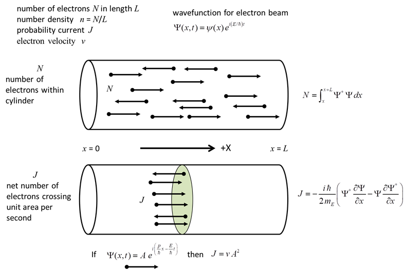
INTRODUCTION

Consider a beam of electrons moving in a [1D] region in which the potential energy is a constant.

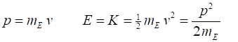
An electron moving under the influence of such a potential energy function is a free particle since the force acting on it is . Hence, the value of the constant for the potential energy is arbitrary. Therefore, we set the potential energy function to zero.

(1)

Each electron in the beam with mass m_E has velocity v , momentum p, kinetic energy K and total energy E

(2)

FREE PARTICLE TRAVELLING WAVES

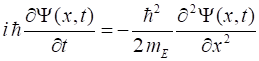
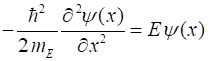
The electron beam wavefunction for a travelling wave free particle which satisfies the Schrodinger wave equations (equations 4A and 4B) can be expressed as

(3)

Time-dependent Schrodinger wave equation

(4A)

Time-independent Schrodinger wave equation

(4B)

For an electron beam travelling to the right (direction of increasing x)

(5)

is called an eigenfucntion

amplitude A

propagation constant (wave number)

angular frequency

de Broglie wavelength

For a free particle the total energy can have any value greater than or equal to zero.

From the uncertainly principle the location of the electrons is “unknown” since the energy and momentum of is assumed to be known.

The probability of finding an electron between x and x+dx is

(6)

As expected, for a uniform electron beam, the probability Prob is not a function of x. The constant A is related to the intensity of the beam. If there are on average N electrons in a length L, we must have

(7)

A stream of electrons constitutes a flow of charged particles and hence an electric current. Such a current can be quantitatively described in terms of wavefunctions. We can define the quantity, J which is called the probability current.

(8)

Simulation of a wave propagating from the left to the right (in the direction of increasing x)

In this example, the wavefunctions are given as mathematical functions. So, it is possible to calculate many properties of the electron beam both analytically and numerically and compare the two sets of values. For example, estimates of the probability current J and amplitudes A and B

Analytical estimate J_max = vA² = 1.1862x10²³ s^-1

Numerical estimate J_max = 1.1860x10²³ s^-1

Input values A = 1x10⁸ and B = 0

Numerical estimate A_n = 1.00x10⁸ and B_n = 1.49x10^-8

For the motion of electrons in non-zero potential fields, the wavefunction is computed by solving the Schrodinger wave equation and so it may be necessary to use purely numerical methods to estimate properties of the beam.

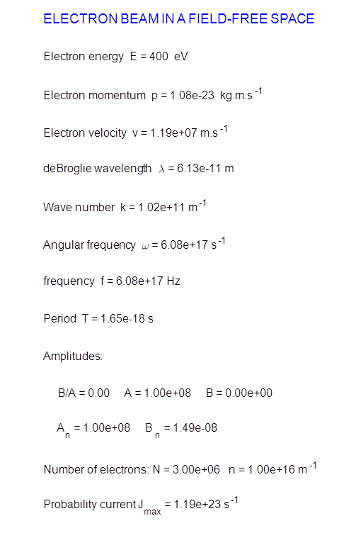
Fig. 1. The simulation input and output parameters are displayed in a Matlab figure Window.

Fig. 2. The wavefunction for an electron beam (E = 400 eV) propagating in the direction of increasing x and the probability current density.

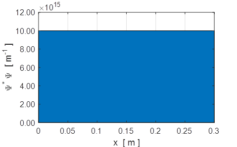
Fig. 3. The probability density function. The area under the graph gives the number of electrons with region of length L = 0.3 nm, N = 3x10⁶. The probability of locating an electron is uniform along the length of the cylinder.

Simulation of a wave propagating from the left to the left (in the direction of decreasing x)

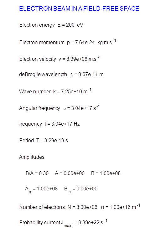
Fig. 4. The simulation input and output parameters are displayed in a Matlab figure Window. Note: The numerical estimates An and Bn are reversed.

Fig. 5. The wavefunction for an electron beam (E = 200 eV) propagating in the direction of decreasing x and the probability current density. Note: the probability current is negative since the electrons are moving to the right.

Fig. 6. The probability density function. The area under the graph gives the number of electrons with region of length L = 0.3 nm, N = 3x10³. The probability of locating an electron is uniform along the length of the cylinder.

FREE PARTICLE STANDING WAVES

We can model the behaviour of the interference of a wave propagating to the right and one to the left.

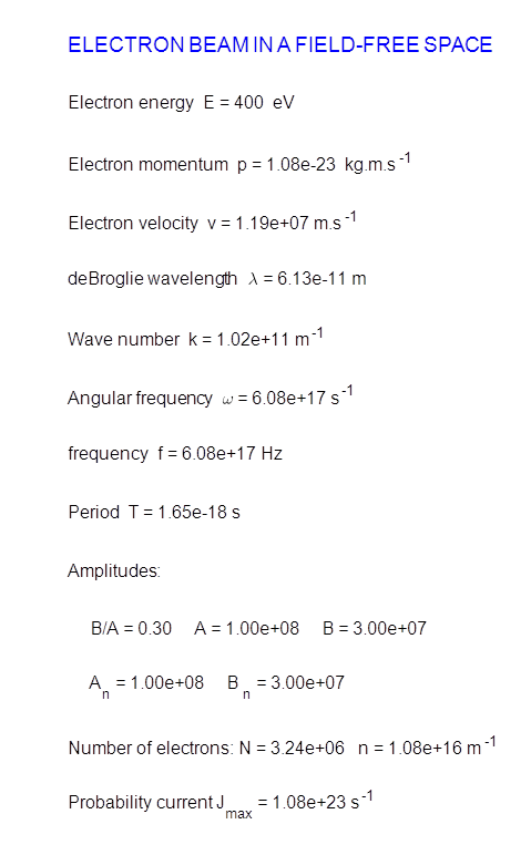
Fig. 7. The simulation input and output parameters are displayed in a Matlab figure Window.

The number of particles N = 3.24x10⁶ in the cylinder is greater than the example shown in figure 1 (N = 3.00x10⁶). This is because we include in the number of particles those that are travelling both to the right and to the left. However, the probability current is less, since the probability current is a measure of the net movement of electrons through a cross-section (1.08x10²³ s^-1 < 1.19x10²³ s^-1).

Fig. 8. The wavefunction for an electron beam (E = 400 eV) which is a superposition of the wavefunctions for the motion to the right and left. The resultant wavefunction is described by a partial standing wave pattern.

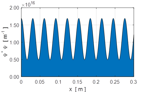
Fig. 9. The probability density function. The area under the graph gives the number of electrons with region of length L = 0.3 nm, N = 3.24x10³. The probability of locating an electron is not uniform along the length of the cylinder. This is a quantum effect and a result that is impossible to explain classically. A partial standing wave pattern is produced due to the interference of the two matter waves propagating in opposite directions. There are distinct region where the waves interfere constructively and where there is a high probability of finding an electron while in other regions, there is a much lower probability due to destructive interference.

If the amplitudes of the two waves are equal A = B, then a pure standing wave pattern is produced where the nodes are fixed in space as shown in figures 10 and 11.

Fig. 10. Animation E = 400 eV: Top: real part of the resultant wave produced by the interference of the two waves moving in opposite directions. Middle: Real part of the wavefunction. Bottom: Imaginary part of the wavelength.

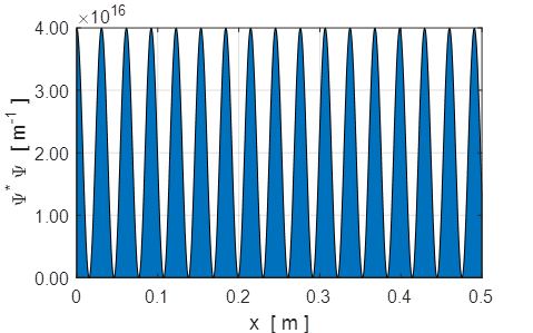
Fig. 11. Probability density function for the standing wave produced by the interference of the two waves of equal amplitude A = B moving in opposite directions. At some location, there is zero probability of locating an electron.

You can easily change the ratio B/A to see the changes in the standing wave pattern.

When an electron beam is incident upon a region where there is a change in the potential energy, then the incident wave may be partially reflected and partially transmitted. The incident and reflected waves will interfere with each other and produce a standing wave as shown in the above example. By calculating the maximum fluctuation of the wavefunction one can then estimate the amplitudes of the incident and reflected waves as was done in the above example using the Script qmElectronBeamA.m.