|
QUANTUM MECHANICS PARTICLE
SCATTERING AND BARRIER PENETRATION ELECTRON BEAMS:
STEP POTENTIAL BEAM ENERGY LESS
THAN STEP HEIGHT E < U0 Ian Cooper matlabvisualphysics@gmail.com |
|
MATLAB SCRIPTS (download files) qmElectronBeamB.m Simulation of an electron matter wave propagating along the X axis which encounters a barrier. The physical system is described with a potential energy function that can be approximated by a step potential. The energy E of the electron beam is less than the step height U0. The simulation input parameters are specified in the INPUT section of the Script % INPUTS
============================================================== % Energy of particles [100 eV]; Es = 50; % Step Potential: height of
step E < U0 [200 eV] U0s = 200; % X axis [-0.5 0.5 nm] xMin = -0.5; xMax = 0.5; % Grid points N = 15501; The Schrodinger wave equation is solved numerically using the Matlab ordinary differential equation solver ode45. There are numerous solutions to this equation. To find a stable solution that does not diverge to infinity it is necessary to perform the integration from the largest to the smallest value of x. The function flip is used to reverse the order of the X grid points. X grid
x = X.*linspace(xMin,xMax,N); ode solver
xSpan = flip(x); u0 =
[1,1i*k]; options
= odeset('RelTol',1e-6); [xR,u] = ode45(@FNode, xSpan, u0, options); The initial conditions
are given by the array u0: u0(1) gives the of the wavefunction and u0(2) the slope of the wavelength.
The slope is given as the imaginary value of the wave number k, where The solver ode45 returns the X grid in reverse order (xR) and the wavefunction and its first derivative (u). The function for the Schrodinger equation is function du = FNode(x,u) global E K U = pot(x); U = U*1.6e-19; y = u(1); ydot = u(2); du = zeros(2,1); du(1) = ydot; du(2) = -K*(E-U)*y; end The step
potential is defined with the function function U = pot(x) % Potential
energy function [eV] global U0s U = 0; if x > 0 U
= U0s; end end The eigenfunction psi, the complex conjugate of the wavefunction psiC and the probability density PD (normalized to 1) are then computed. % Eignenfunction psi = u(:,1); psiS = conj(psi); psi_max =
max(real(psi)); % Probability Density PD = conj(psi).*psi; PD =
PD./max(PD); The de Broglie
wavelength of the electron matter is given by The de Broglie
wavelength % Numerical estimate of wavelength from peak #2 and peak
#(N-1) [pks, locs] = findpeaks(real(psi),x); LEN = length(locs); wL_N = (locs(3) - locs(2) ) / (1); where You can compare the two values of the wavelength to check the validly of the numerical solution.
The propagation of the waves is animated, and the animation can be saved as a gif file by setting f_gif = 1. The time dependent wavefunction is
The X and Y coordinates for the animated plot are:
xP = xR./X;
yP = real(psi) .* real(psiT(c));
|
|
STEP POTENTIAL E < U0 In this article, we shall investigate the solutions of
the time-independent Schrodinger wave equation for an electron where the
potential energy
(1)
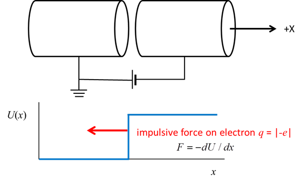
This is an idealized potential which approximates many potentials that occur in real situations. The results we obtain using our idealized potential illustrate a number of characteristic quantum mechanical phenomena. We may think of
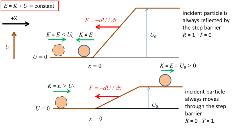
Fig. 1. Step potential function. The electron moves along the X axis of two cylindrical electrodes held at different voltages. The potential energy of the system is constant when an electron is inside either electrode, but changes rapidly when passing from one to the other. A step potential is a good approximation for the motion a conduction electron moving near the surface of a metal. For a classical particle, the subsequent motion when it impacts the step barrier depends on the kinetic energy of the classical particle and the height of the barrier as shown in figure 2.
Fig. 2. The total energy of a classical
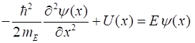
particle is conserved, To determine the motion of the electron according to quantum mechanics, we must find a solution of the time independent Schrodinger equation, since the potential energy function is independent of time. We can solve the Schrodinger equation (equation 2) numerically using the Matlab ordinary differential equation solver ode45. It is often much easier to solve the Schrodinger equation numerically, rather than doing lots of algebra to get an analytical solution. Also, for more realistic potentials energy functions, there are no analytical solutions. (2) where
the solution is the eigenfunction
(3) The Script qmElectronBeamB.m solves the
Schrodinger equation (equation 2) for the case where an electron beam is
incident upon the step barrier with total energy which is less than the
height of the barrier
(4)
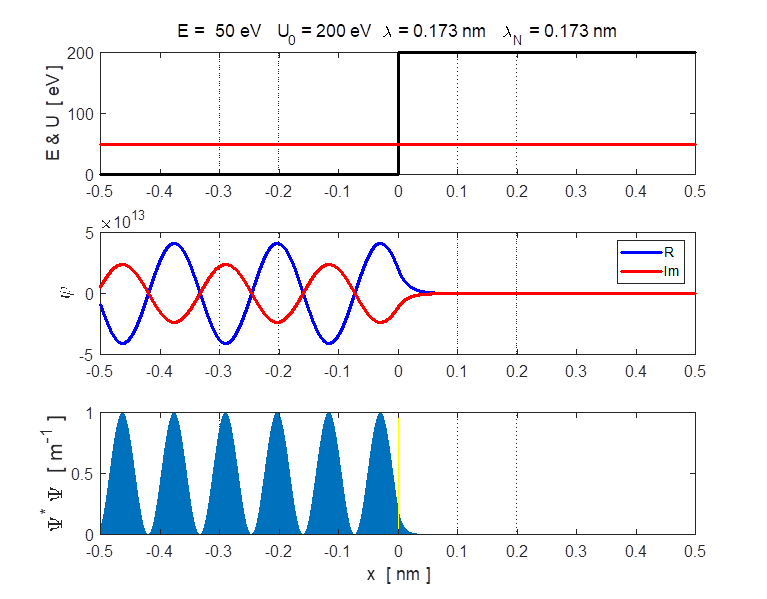
Figure 2 show an animation of the real part of the wavefunction. The wavefunction has been normalized so that its maximum amplitude is 1.
Fig. 2. E
= 50 eV and U0
= 200 eV. Real part of the wavefunction
Fig. 3. Plots of the potential energy
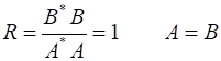
function, the real and imaginary parts of the eigenfunction The solution of the Schrodinger equation is that of a standing wave as shown in figures 2 and 3. It is a combination of an incident wave travelling to the right and a reflected wave travelling to the left. The two propagating waves moving in opposite directions are of equal intensities since the nodes are stationary points and the normalized probability distribution varies from 0 to 1. Hence, the amplitude of the incident wave is A and the amplitude of the reflected wave is B, must be equal, A = B. At a potential step (x = 0), the wave is either reflected or transmitted from the barrier. The reflection coefficient is R and the transmission coefficient is T. The reflection coefficient is equal to the ratio of the intensity of that part of the wave that describes the reflected particle to the intensity of that part that describes the incident particle. The transmission coefficient is equal to the ratio of the intensity of that part of the wave that describes the transmitted particle to the intensity of that part that describes the incident particle. Since there is no absorption of energy, R + T = 1
In the case where E < U0, the two waves of the same amplitude are moving at the same speed but in opposite directions. Hence the reflection coefficient R is
(5)
Therefore, the transmission coefficient must be zero, T = 0. The fact that R = 1 means that a particle incident upon the potential step with total energy less than the height of the step, has a probability of one of being reflected, - it is always reflected. This is in agreement with the predictions of classical physics. In the region x
> 0, the probability density is very small and decreases rapidly with
increasing x. Hence, there
is a finite probability of finding the electron in the region x > 0. In terms of classical
physics, it would be absolutely impossible to find the electron in the region
x > 0 because there the
total energy is less than the potential energy, so the kinetic energy
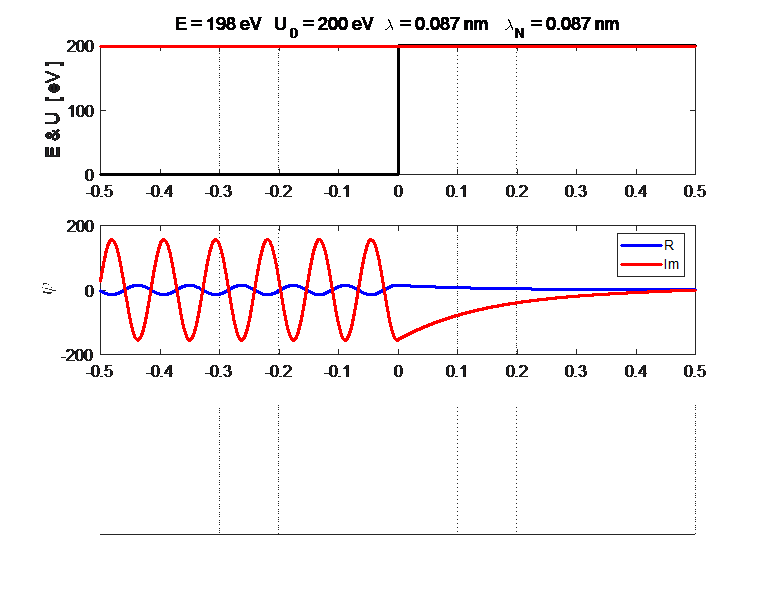
Fig. 4. Fig. 2. E
= 198 eV and U0
= 200 eV. Real part of the wavefunction
Fig. 5. Plots of the potential energy
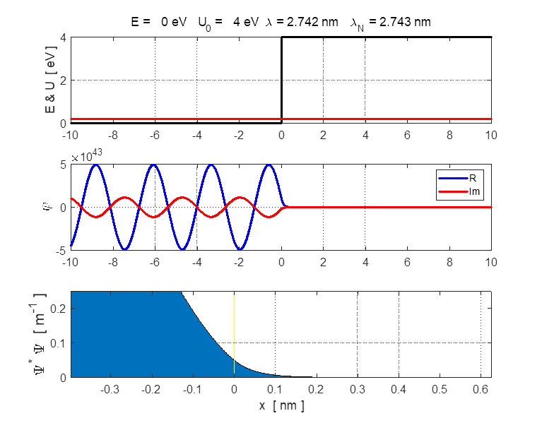
function, the real and imaginary parts of the eigenfunction Example A conduction electron moves through a block of copper with total energy E = 0.2 eV. To a good approximation, the surface acts like a step barrier of height 4.0 eV. This step barrier bounds the electron within the metal. We can estimate the penetration distance using the following input parameters:
E = 0.2 eV U0 = 4.0 eV
xMin = -10 nm xMax
= 10 nm Figure 6 shows an enlarged view of the probability density function. The penetration distance into the classically forbidden region is about 0.1 nm. This penetration distance is of the order of atomic dimensions. This penetration effect has very important consequences in atomic and nuclear systems.
Fig. 6. Enlarged plot of the probability density function using the zoom function. The penetration distance is in the order of 0.1 nm. |