DOING PHYSICS WITH MATLAB

QUANTUM PHYSICS

SCHRODINGER EQUATION

Time evolution of the wavefunction  -  stationary and compound states

Ian Cooper

matlabvisualphysics@gmail.com

DOWNLOAD DIRECTORY FOR MATLAB SCRIPTS

The Matlab scripts are used to give the solution of the Schrodinger Equation for a variety of potential energy functions using a matrix method where the solutions are the eigenvalues and eigenfunctions of the energy operator. Read the paper on the Matrix Method before proceeding with this paper.

se_wells.m

First m-script to be run when solving the Schrodinger Equation using the Matrix Method. Most of the constants and all the well parameters are declared in this file. You can select the type of potential well from the Command Window when the m-script is run.  You alter the m-script code to change the parameters that characterize the wells and you can add to the m-script to define your own potential well. When this m-script is run it clears all variables and closes all open Figure Windows.

se_solve.m

This m-script solves the Schrodinger Equation using the Matrix Method after you have run the m-script se_wells.m. The eigenvalues and corresponding eigenvectors are found for the bound states of the selected potential well.

se_stationary.m

To be run after se_wells.m and se_solve.m. You can investigate and view the time evolution of an energy eigenstate and save the plot as an animated gif.

se_super.m

To be run after se_wells.m and se_solve.m. You can investigate and view the time evolution of a compound state and save the plot as an animated gif.

STATIONARY STATES AND SUPERPOSITION PRINCIPLE

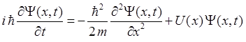
In wave mechanics, the state of a system is described by a wavefunction that satisfies the Schrodinger Equation and the boundary conditions imposed on the system. For a one dimensional system, the Schrodinger Equation for a potential energy function U(x) is

         (1)        

We will consider only those solutions that are described by a state of definite energy by the method of separation of variables where the wavefunction is expressed as

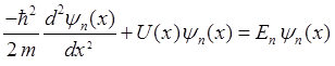
         (2)        

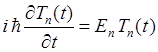
The substitution of this wavefunction into the Schrodinger Equation, gives two ordinary differential equations and for quantum state n

         (3)         time independent Schrodinger equation

         (4)         n = 1, 2, 3 , …     

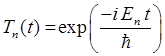
The solution of the ordinary differential equation (4) is

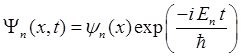
         (5)        

For stationary states which have a definite total energy, the wavefunction is

         (6)        

If the energy of the system is measured, the value E_n will certainly be obtained. This is a special type of solution of the Schrodinger Equation.

Applying Born’s rule, which states that the probability of finding the particles in a small interval dx centered on x for the state n is

Hence, the probability is independent of time t and this is why it is called a stationary state. The real and imaginary parts of the wavefunction change with time but not the modulus. All parts oscillate in phase (like a stationary normal mode of a vibrating guitar string). The concept of stationary states is not one that is familiar to us in the classical world as nothing is moving at all, the probability of detecting an electron in any given region never changes. 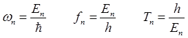All the expectation value such as position, momentum and energy are also independent of time.

Each stationary state wavefunction as described by equation (6) describes a complex standing wave. A standing wave is one that oscillates without propagation through space, with all points of the standing wave vibrating in phase. The frequency and period of the vibration are

The standing wave has nodes fixed in space. As n increases, the total energy E_n and number of nodes increases, while the period of vibration T_n decreases.

There is zero probability of locating the particle bound in the well at each node. We can no longer think of the particle moving from place to place in the well. In quantum physics, a particle has no position until it is measured, so it makes no sense to think of the particle moving about. There is no problem associated with the particle having to travel through a nodal point, since the particle has no position and velocity. When a measurement is made, it only tells us the position and velocity at the instant after the measurement. 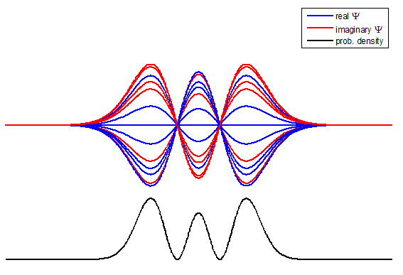Before the measurement, the state is simply described by the wavefunction which gives us the most complete description that is possible of the state of the system, but it does not give us information about the position and velocity of the particle.

Figure (1) show the time evolution for a number of time steps of the real and imaginary parts of the wavefunction and the probability density for the stationary state n = 3 of the truncated harmonic oscillator. The phase of the real and imaginary parts change with time but the probability density is independent of time.

         Fig. 1. The time evolution of the wavefunction’s real and imaginary parts for the stationary state n = 3 for a truncated parabolic well. The probability density does not change with time.

[se_wells.m se_solve.m se_stationary.m]

An animation of the changes with time of the wavefunction can be observed by running the m-script se_stationary.m.

          Fig. 2. An animated gif of the time evolution of the stationary state n = 3 for a truncated parabolic well. [se_stationary.m]

Wavefunctions have a very important property in that they obey the superposition principle:

If a set of wavefunctions are solutions of the Schrodinger Equation, then any linear combination of the wavefunctions is also a solution

     where a_c are arbitrary complex numbers

If the wavefunctions are normalized wavefunction and is also normalized then

The probability density of finding a particle in a given length element dx is

When the particle is in an eigenstates with a definite energy E_n then

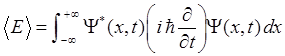
and so the probability distribution does not change with time as shown in figure (1). Also, the expectation value for the position of the particle  is not a function of time. However, when the particle is in a compound state (more than one a_n is nonzero), the probability density , the expectation value for position and probability of locating the particle at each position all vary with time.

The expectation value for the total energy is

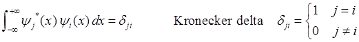
Using the fact that the eigenfunctions are orthonormal

and doing some algebra it is not difficult to show that the expectation value for the total energy is

         (7)                   where E_c are the eigenvalues

Any measurement of the total energy of the system will always give one of the eigenvalues E_n and not . If many identical system with the compound wavefunction were prepared and the total energy measured for each system than the average value those measurements would be very close to the expectation value .

Run se_wells.m and se_solve.m for the default truncated parabolic well:

% parabolic *****************************************************

case 5  

xMin = -0.2;                  % default = -0. nm

xMax = +0.2;                  % default = +0.2 nm

    x1 = 0.2;                     % width default = 0.2 nm;

    U1 = -400;                    % well depth default = -400 eV;

The energy eigenvalues for this potential well from se_solve.m are:

No. bound states found =  5  

 Quantum State / Eigenvalues  En  (eV)

  1      -360.92  

  2      -282.77  

  3      -204.68  

  4      -127.09  

  5      -52.272 

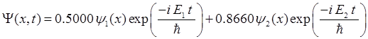
The m-script se_super.m adds any two of the eigenfunctions to form a compound state. To investigate the addition of the eigenstates 1 and 2, in the code for se_super.m enter

qn(1) = 1; qn(2) = 2;       % states to be summed

ac(1) = 0.5; ac(2) = sqrt(1-ac(1)^2);     % coefficients 

to form the compound state

         (8)         

The expectation value (eV) for this compound state is displayed in the Command Window

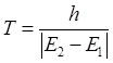
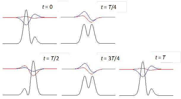
Eavg_s =  -302.3036          see equation (7)

Figure (3) shows the time evolution of the compound state at times t = 0, T/4, T/2, 3T/4, T  where T is the period of the oscillation of the wavefunction. The red curves are the real parts and the blue curves the imaginary part of the compound wavefunction. The black curves shows the variation with time of the probability density. For the compound state where the probability curve oscillates back and forth in the potential well with a period T where            

         Fig. 3.    The time evolution of the wavefunction’s real and imaginary parts for a compound state given by equation (8) for a truncated parabolic well. The probability density changes with time as the charge distribution oscillates back and forward in the potential well. Red curves – real part , blue curves – imaginary partand black curves – probability density.

[se_wells.m se_solve.m se_super.m]

        Fig. 4. An animated gif of the time evolution of the compound state n = 1 and n = 2 for a truncated parabolic well.

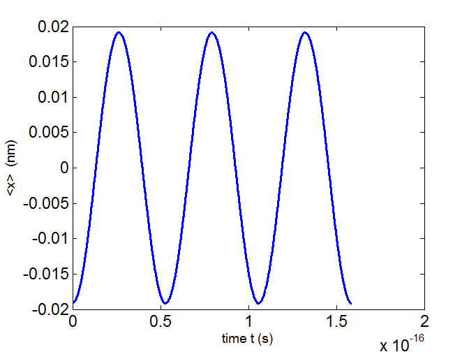
[se_super.m]

Therefore, the expectation of the position of the electron oscillates with the period T as shown in figure (5).

         Fig. 5.    The time variation of the expectation value for the position of the electronin the compound state

state n = 1 and n = 2 for a truncated parabolic well. T = 5 .294×10^-17 s.    [se_wells.m se_solve.m se_super.m]

RADIATION EMITTED BY THE SYSTEM

In classical electromagnetism, an accelerated charge radiates electromagnetic radiation at a rate that increases with its acceleration. In quantum mechanics, the acceleration of a particle is not defined and an electron in a given state does not radiate energy. But, we can explain the radiation due to transitions between states using a semi-classical approach by considering the expectation value instead of the classical well defined position coordinate x. Consider an electron in a stationary eigenstate. Its expectation value does not depend upon time

therefore,  and no energy is radiated.

So, a stationary state does not radiate. However, the bound particle is not alone in the universe, sooner or later the particle will interact with its surroundings (photon, or some other particle, etc), perturbing the energy so that the particle is no longer in a stationary state. The particle will start in its initial stationary state, absorb a photon for example, and then exist in a compound state where the coefficients a_n are now time dependent. In the compound state, the system does not have a definite energy and the expectation value is now time dependent. Finally a transition will occur to a lower energy eigenstates and a photon will be emitted. The product  where q is the charge on the particle is the x component of an oscillating electric dipole moment for which the frequency of the radiation emitted is

For the our compound state in the harmonic potential well, the variation the expectation values with time depends on the exponential term

and the expectation valuevaries with time as shown in figure (5) because of the variation with time of the probability distribution. The frequency of oscillation of is y given by . Hence, the frequency of the emitted photon is the same as the frequency at which the charge distribution changes. Assume that the initial state of the system is the eigenstates n = 2 and E₂ = 282.7 eV. Then system is disturbed to produce the compound state given by equation (8).  In this complex state, the charge distribution oscillates with a frequency f₂₁ and finally a photon is emitted with frequency f₂₁ as the system loses energy and returns to the ground state

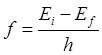
n = 1, E₁= - 360.92 eV. The values of the frequency and wavelength of the emitted photon for the transition are:

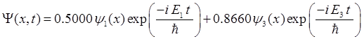
n = 2 à n = 1     Dn = +1       f₂₁ = 1.89×10¹⁶ Hz         l₂₁ = 1.59×10^-8 m   (UV)

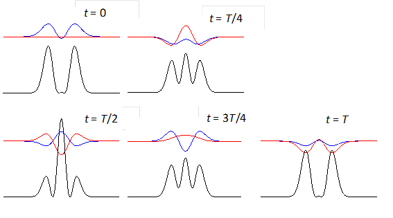
We will now consider the compound state which is a summation of the two eigenstates n = 1 and n = 3

            (9)      

The time evolution of the real and imaginary parts of the wavefunction and the probability density are shown in figure (6). However, even though the probability density changes with time, there is no sloshing back and forward and the expectation value for position as . Therefore, no radiation can be emitted in the transition n = 3 à n = 1 for our harmonic oscillator potential well. So, in the case of the one-dimensional harmonic oscillator, electric dipole radiation is emitted when n decreases by 1 and absorbed only when n increases by 1. Thus, the harmonic oscillator obeys the selection rule , and the only frequency emitted or absorbed is the classical oscillator frequency since the energy levels are equally spaced¸ where

m         mass of particle

k_s         spring constant for system

         Fig. 6.    The time evolution of the wavefunction’s real and imaginary parts for a compound state given by equation (9) for a truncated parabolic well. The probability density changes with time as the charge distribution oscillates back and forward in the potential well. Red curves – real part , blue curves – imaginary partand black curves – probability density.

[se_wells.m se_solve.m se_super.m]

        Fig. 7.  An animated gif of the time evolution of the compound state n = 1 and n = 3 for a truncated parabolic well.

       The time variation of the expectation value for the position of the electronis =  0.

[se_wells.m se_solve.m se_super.m]

Investigations

Run se_wells.m, se_solve.m and then se_stationary.m and explore the characteristics of the time evolution of stationary states. Determine the frequency and period of the oscillations.

Run se_wells.m, se_solve.m and then se_super.m and explore the characteristics of compound wavefunctions.

Select the truncated harmonic potential well and verify that radiation is emitted only for transitions where .