DOING PHYSICS WITH MATLAB

[1D] TIME DEPENDENT SCHRODINGER EQUATION:

PROPAGATION OF A FREE PARTICLE

Ian Cooper

matlabvisualphysics@gmail.com

DOWNLOAD DIRECTORY FOR MATLAB SCRIPTS

sefdtdA.m

The script is used to solve the [1D] time dependent Schrodinger equation using the finite difference time development method for the propagation of a wave packet that represents a free particle (electron). Animations of the time evolution of the wavefunction (real and imaginary parts and phase) and the probability density are displayed graphically. Animations are saved as an animated gif file. You can easily modify the script to save the animations as an avi file. Also, various expectation values are computed for the initial state and final state of the particle. The script calls two external functions simpson1d.m which is used to evaluate the integrals for the expectation values and colorCode.m which is used to specify the colour for the phase of the complex wave function.

PROPAGATION OF A FREE PARTICLE

Using the finite different time development method, the [1D] time dependent Schrodinger equation can be solved to the show the propagation of a wave packet that represents the motion of a particle in real-space and real-time. The wave packet is specified by a sinusoidal function with wavelength and a Gaussian envelope.

Figure 1 shows an animation of the motion of an electron in free space as it travels in a positive X-direction and figure 2 shows the propagation of the particle’s probability density function and the phase of the wavefunction indicated by colour. A summary of the simulation parameters is displayed in Matlab Figure Window as shown in figure 3.

Fig. 1. Animation of a particle propagating in free space. The imaginary part of the wavefunction leads the real part. This results in the direction of propagation of the wave to be in the +X direction.

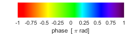
Fig. 2. Time evolution of the probability density and the phase of the wavefunction. The phase of the complex wavefunction is specified by a colour.

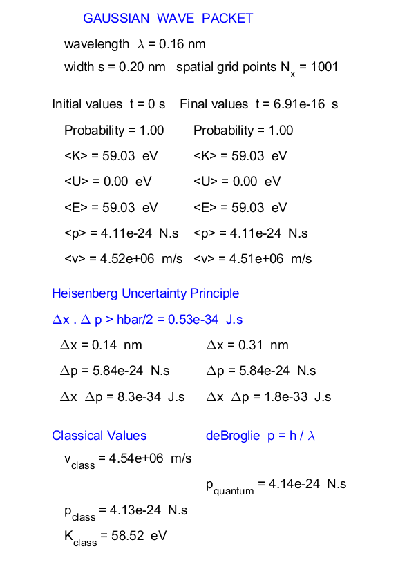
Fig. 3. A summary of the simulation parameters are displayed in a Matlab Figure Window.

The peak of the probability density function propagates according to the rules of classical physics with the speed of propagation given by . The momentum and kinetic energy of the particle are and . For the free propagation of the wave packet (particle), the total energy of the particle is conserved. The classical prediction for the momentum agrees with the momentum of the particle given by the de Broglie relationship .

As the wave packet propagates its width steadily increases. This is shown by the increasing value of the expectation value for the position . According to classical physics the position of the particle and its momentum have definite values at all times. However, according to the principles of quantum mechanics, at each instant, we only can compute the probability of locating the particle and the expectation values and the uncertainties for position and momentum. The results of the simulation calculations show that indeed the Heisenberg Uncertainty relationship is satisfied.

In script, the real part of the wavefunction is calculated at times . However, the imaginary part of the wavefunction is calculated at times . So, the imaginary part of the wavefunction is modified:

Alternatively, if this is not done, the calculations can be done at integer and half-integer time steps. For example, the probability density

The animation of the phase in Figure Window 3 using the area function runs extremely slowly. Don’t know why.