|
THERMAL PHYSICS BLACKBODY
RADIATION Ian Cooper |
|
MATLAB SCRIPTS (download files) The
continuous spectrum of a blackbody at different temperatures can be
investigated. tpSun.m Simulation
of the electromagnetic radiation emitted from the Sun. The Script can be used
to create colour spectrums of the radiation emitted
from the Sun by calling the Script Colorcode.m. tpStar.m Simulation
of the blackbody curve of a star. You can change the temperature of the star
and observe its blackbody temperature. The Script can be used to create colour spectrums of the radiation emitted from a star Sun
by calling the Script Colorcode.m. tpFilament.m Simulation
of the radiation emitted by a hot tungsten filament. tpBlackbody.m Simulation
of the radiation emitted from a hot object at four temperatures. simpson1d.m Function
to evaluate the area under a curve using Simpson’s 1/3 rule. ColorCode.m Function
to return the appropriate colour for a wavelength
in the visible range from 380 nm to 780 nm. |
|
THERMAL RADIATION
AND BLACKBODIES PARTICLE NATURE OF
ELECTROMAGNETIC RADIATION The wave
nature of electromagnetic radiation is demonstrated by interference
phenomena. However, electromagnetic radiation also has a particle nature. For
example, to account for the observations of the radiation emitted from hot
objects, it is necessary to use a particle model, where the radiation is
considered to be a stream of particles called photons. The energy of a photon, E is (1) The
electromagnetic energy emitted from an object’s surface is called thermal radiation and is due a decrease in
the internal energy of the object. This radiation consists of a continuous
spectrum of frequencies extending over a wide range. Objects at room
temperature emit mainly infrared and it is not until the temperature reaches
about 800 K and above that objects glows visibly. A blackbody is an object that
completely absorbs all electromagnetic radiation falling on its surface at
any temperature. It can be thought of as a perfect absorber and emitter of
radiation. The power emitted from a blackbody, P is given by
the Stefan-Boltzmann
law and it depends only on the surface area of the emitter, A and its
surface temperature, T (2) A more
general form of equation (2) is (2) where e is the emissivity of the object. For a blackbody, e = 1. When e < 1 the object is called a graybody
and the object is not a perfect emitter and absorber. The amount
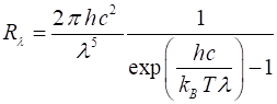
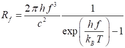
of radiation emitted by a blackbody is given by Planck’s radiation law and is
expressed in terms of the spectral exitance for wavelength or frequency
Rl or Rf respectively (4) or (5) In the
literature, many different terms and symbols are used for the spectral exitance. Sometimes the terms and the units given are
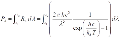
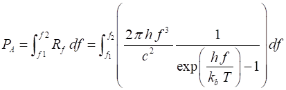
wrong or misleading. The power radiated per unit surface of a blackbody, PA within
a wavelength interval or bandwidth, (l1, l2) or frequency
interval or bandwidth (f1,
f2) are given by
equations 6 and 7 (6) and (7) The
equations 6 and 7 give the Stefan-Boltzmann law (equation 2) when the
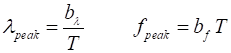
bandwidths extend from 0 to ¥. Wien’s Displacement law states that
the wavelength lpeak
corresponding to the peak of the spectral exitance
given by equation 4 is inversely proportional to the temperature of the
blackbody and the frequency fpeak for the
spectral exitance peak frequency given by equation
5 is proportional to the temperature (8)
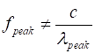
The peaks
in equations 4 and 5 occur in different parts of the electromagnetic spectrum
and so (9) The
Wien’s Displacement law explains why long wave radiation dominates more
and more in the spectrum of the radiation emitted by an object as its
temperature is lowered. When
classical theories were used to derive an expression for the spectral exitances Rl and Rf, the power emitted by a blackbody diverged to infinity as the
wavelength became shorter and shorter. This is known as the ultraviolet catastrophe. In 1901 Max Planck proposed a
new radical idea that was completely alien to classical notions,
electromagnetic energy is quantized.
Planck was able to derive the equations 4 and 5 for blackbody emission and
these equations are in complete agreement with experimental measurements. The
assumption that the energy of a system can vary in a continuous manner, i.e.,
it can take any arbitrary close consecutive values fails. Energy can only
exist in integer multiples of the lowest amount or quantum, h f. This step marked
the very beginning of modern quantum theory. A summary of the physical quantities, units and values of constants used in the description of the radiation from a hot object. |
Variable |
Interpretation |
Value |
Unit |
|
E |
energy of photon |
|
J |
|
h |
Planck’s constant |
6.62608´10-34 |
J.s |
|
c |
speed of electromagnetic radiation |
3.00x10⁸ |
m.s-1 |
|
f |
frequency of electromagnetic
radiation |
|
Hz |
|
l |
wavelength of electromagnetic
radiation |
|
|
|
T |
surface temperature of object |
|
K |
|
A |
surface area of object |
|
m2 |
|
s |
Stefan-Boltzmann constant |
5.6696´10-8 |
W.m-2.K-4 |
|
P |
power emitted from hot object |
|
W |
|
e |
emissivity of object’s
surface |
|
|
|
Rl |
spectral exitance:
power radiated per unit area per unit wavelength interval |
|
(W.m-2).m-1 |
|
Rf |
spectral exitance:
power radiated per unit area per unit frequency interval |
|
(W.m-2).s-1 |
|
kB |
Boltzmann constant |
1.38066´10-23 |
J.K-1 |
|
bl |
Wien constant: wavelength |
2.898´10-3 |
m.K |
|
bf |
Wien constant: frequency |
2.83
kB T / h |
K-1.s-1 |
|
lpeak |
wavelength of peak in solar
spectrum |
5.0225´10-7 |
m |
|
RS |
radius of the Sun |
6.96´108 |
m |
|
RE |
radius of the Earth |
6.96´106 |
m |
|
RSE |
Sun-Earth radius |
6.96´1011 |
m |
|
I0 |
Solar constant |
1.36´103 |
W.m-2 |
|
a |
Albedo of Earth’s surface |
0.30 |
|
|
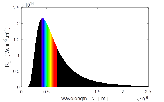
SIMULATION: THE
SUN AND THE EARTH AS BLACKBODIES Inspect and run the Script tpSun.m so that
you are familiar with what the program and the code does. The Script calls
the functions simpson1d.m and Colorcode.m. The Sun can
be considered as a blackbody, and the total power output of the Sun PS can be
estimated by using the Sefan-Boltzmann law,
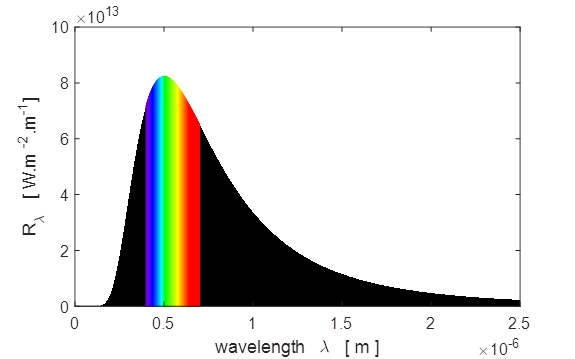
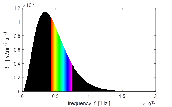
equation 2, and by finding the area under the curves for Rl and Rf using
equations 6 and 7. From observations on the Sun, the peak in the
electromagnetic radiation emitted has a wavelength, lpeak = 502.25 nm (yellow). The temperature of the Sun’s
surface (photosphere) can be estimated from the Wien displacement law,
equation 8. The
distance from the Sun to the Earth, RSE can be used
to estimate of the surface temperature of the Earth TE if there
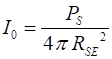
was no atmosphere. The intensity of the Sun’s radiation reaching the
top of the atmosphere, I0 is known as
the solar constant (10) The power
absorbed by the Earth, PEabs is (11) where a is the
albedo (the reflectivity of the Earth’s surface). Assuming the Earth
behaves as a blackbody then the power of the radiation emitted from the
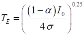
Earth, PErad is (12) It is known
that the Earth’s surface temperature has remained relatively constant
over many centuries, so that the power absorbed and the power emitted are
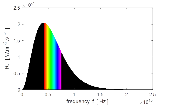
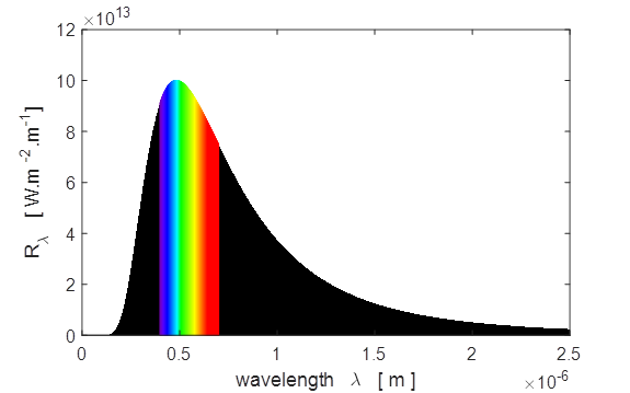
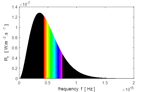
equal, so the Earth’s equilibrium temperature TE is (13) Sample results using tpSun.m Plots of the spectral exitance curves
Matlab screen output for sun.m Sun: temperature of photosphere, T_S =
5770 K Peak in Solar Spectrum Theory: Wavelength
at peak in spectral exitance, wL
= 5.02e-07 m Graph: Wavelength at peak in spectral exitance, wL = 5.04e-07 m
Corresponding
frequency, f = 5.95e+14 Hz Theory: Frequency
at peak in spectral exitance, f = 3.39e+14 Hz Graph: Frequency at peak in spectral exitance, f = 3.40e+14 Hz Corresponding
wavelength, wL = 8.82e-07 m
Total Solar Power Output P_Stefan_Boltzmann
= 3.79e+26 W P(wL)_total =
3.77e+26 W P(f)_total
= 3.79e+26 W IR
visible UV P_IR =
1.92e+26 W Percentage IR radiation = 51.0 P_visible
= 1.39e+26 W Percentage visible
radiation = 36.8 P_UV =
4.61e+25 W Percentage UV
radiation
= 12.2 Sun - Earth Theory: Solar
constant I_O = 1.360e+03 W/m^2 Computed: Solar
constant I_E = 1.342e+03 W/m^2 Surface temperature
of the Earth, T_E = 254 K
Surface temperature
of the Earth, T_E = -19 deg C Questions 1 How
do the peaks in the plots Rl and Rf compare with the
predictions of the Wien displacement law and lpeak = 502.25
nm (yellow). 2 Compare
the total solar power emitted by the Sun calculated from the Stefan-Boltzmann
law and by the numerical integration to find the area under the spectral exitance (Rl and Rf)
curves. 3 Compare
the percentage the radiation in the ultraviolet, visible and infrared parts
of the solar spectrum. 4 How
does the computed value of the intensity of the radiation reaching the
Earth’s surface, IE compare
with the solar constant, I0? 5 From
our simple model, the surface temperature of the Earth was estimated to be
-19 oC. Is this sensible? What is
the surface temperature on the moon? The average the temperature of the Earth
is much higher than this, about +15 oC.
Explain the difference. 6 What
changes occur in the calculations if the Sun was hotter (peak in the blue
part of the spectrum) or cooler (peak in the red) part of the spectrum? 7 What
would be wavelength lpeak and the
temperature of the Sun’s surface if the Earth’s equilibrium
temperature was -15 oC instead -19 oC? (In the m-script, increase the value of lpeak until you reach
the required equilibrium temperature of the Earth.) M-script
highlights 1 Suitable
values for the wavelength and frequency integration limits for equations (6)
and (7) are determined so that the spectral exitances
at the limits are small compared to the peak values. 2 The
Matlab function area is
used to plot the spectral exitance curves, for
example, in plotting the Rl curve: h_area1
= area(wL,R_wL); set(h_area1,'FaceColor',[0
0 0]); set(h_area1,'EdgeColor','none'); 3 The
color for the shading of the curve matches that of the wavelength in the
visible part of the spectrum. A call is made to the function ColorCode.m
to assign a color for a given wavelength band. For the shading of the Rl curve: thisColorMap = hsv(128); for
cn = 1 : num_wL-1 thisColor = ColorCode(wL_vis(cn)); h_area = area(wL_vis(cn:cn+1),R_wL_vis(cn:cn+1)); set(h_area,'FaceColor',thisColor); set(h_area,'EdgeColor',thisColor); 4 Simpson’s
1/3 rule is used for the numerical integration (simpson1d.m) to find the area under the spectral
intensity curves. For the Rl curve, the total power radiated by the Sun: P_total = A_sun *
simpson1d(R_wL,wL1,wL2); 5 The
peaks in spectral intensities are calculated using Matlab logical functions: wL_peak_graph
= wL(R_wL == max(R_wL)); f_peak_graph
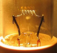
= f(R_f == max(R_f)); SIMULATION: HOW EFFICIENT IS A HOT TUNGSTEN FILAMENT ?
Inspect and run the Script tpFilament.m so that you are familiar with what
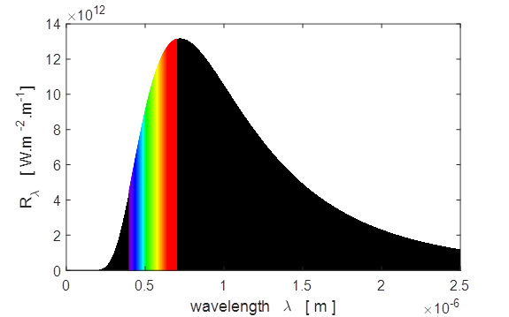
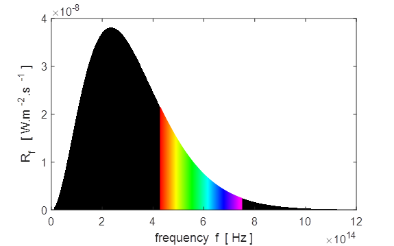
the program and the code does. The Script calls the functions simpson1d. Some car headlights use a hot tungsten filament to emit
electromagnetic radiation. We can estimate the percentage of this radiation
in the visible part of the electromagnetic spectrum for a hot tungsten
filament that has a surface temperature of 2400 K and an electrical power of
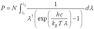
55 W (the thermal power radiated is also 55 W). The first step is to
calculate the thermal power radiated P by a hot object using equation 14
(14) where N is a normalizing
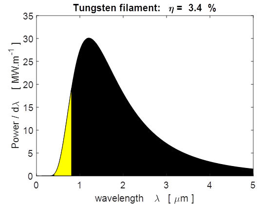
constant and includes a factor for the surface area such that P = 55 W. The
area under the power per unit wavelength curve is shaded yellow to show the
visible part of the spectrum. Lastly, the function Rl is
numerical integrated for the limits corresponding to only the visible part of
the electromagnetic spectrum l1 = 700 nm
(red) and l2 = 400 nm
(blue) This
gives only the total power radiated in the visible part of the
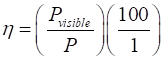
electromagnetic spectrum, Pvisible. The
filament efficiency, h given as
percentage of visible radiation emitted by the hot tungsten filament to the
power consumed by the filament
(16) Sample Results for
tpFilament.m
Matlab screen
output
wavelength at peak =
1.21e-006 m
wavelength at peak =
1.21 um
P_total
= 55.0 W
P_visible =
1.9 W
efficiency (percentage) =
3.5
Check
normalization P_check
= 55.0 W Questions 1 Are
your surprised by the efficiency of the tungsten filament used in a light
globe? 2 What
part of the electromagnetic spectrum does the peak in the spectral intensity
curve occur? 3 Most
of the energy emitted from the light globe is not emitted in the visible part
of the electromagnetic spectrum. What happens to most of the electrical
energy supplied to the light globe? 4 What
temperature would the filament have to be at so that the peak is in the
visible part of the spectrum? Is this possible? 5 What
is the minimum temperature of the filament so that the globe just starts to
glow? 6 How
do the results change if the power emitted by the hot tungsten filament was
75 W? SIMULATION:
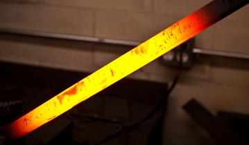
THERMAL RADIATION EMITTED FROM A HOT OBJECT Inspect and run the Script tpBlackbody.m so that you are
familiar with what the program and the code does. The Script calls the
function simpson1d.m for the
numerical integration to compute the power emitted from the spectral exitance function.
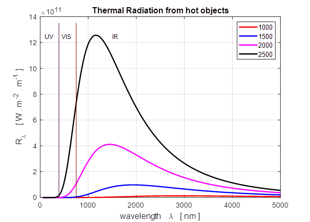
What part of the rod is at the highest temperature? The thermal radiation emitted by a blackbody at four different
temperatures is modeled. The spectral exitance
curves for each temperature are plotted. Notice that even a temperatures as
high as 2000 K only a small amount of radiation is emitted in the visible
part of the electromagnetic spectrum. From the graphical output and the numerical
values displayed in the Command Window, it is easy to verify that the
Stefan-Boltzmann Law and the Wien’s Displacement Law are satisfied. A table can be displayed in Command Window using the Matlab table function. The centre
column is the relative power emitted by the hot object. You can see that when
the temperature is doubled, the power emitted increases by a factor of 16 (24)
and the peak wavelength in the blackbody curve is inversely proportional to
the surface temperature of the object. disp(' '); CWT
= table(T,round(P,2),round(wL_Peak,0), 'VariableNames', {'T [K]', 'Prel',
'wL_Peak [nm]'}); disp(CWT) disp(' ')
T [K] Prel wL_Peak
[nm]
_____
_____
___________
1000 1
2898
1500
5.08
1932
2000
16.07 1449
2500
39.25
1159
SIMULATION: STAR TEMPERATURES Inspect and run the Script tpStar.m so that you are
familiar with what the program and the code does. The Script calls the
function simpson1d.m for the
numerical integration to compute the power emitted from the spectral exitance function. The star temperature is entered in the
INPUT section of the Script. Stars
approximate blackbody radiators and their visible color depends upon the
temperature of the radiator. The curves below are for a blue, a yellow-white, and a red star.
The yellow-white star has a colour is like our Sun.
Blue Star Star:
temperature of photosphere, T_S = 7000 K Peak
in Star Spectrum Theory: Wavelength at peak in
spectral exitance, wL =
414 nm Graph: Wavelength at peak in spectral exitance, wL = 415 nm Correspondending
frequency, f = 7.22e+14 Hz Theory: Frequency at peak in
spectral exitance, f = 4.11e+14 Hz Graph: Frequency at peak in spectral exitance, f = 4.13e+14 Hz Correspondending
wavelength, wL = 7.27e-07 m
Total
Solar Power Output P(wL)_total =
1.35e+08 a.u.
IR visible UV P_IR =
5.09e+07 W Percentage IR
radiation
= 37.6 P_visible
= 5.35e+07 W Percentage visible radiation =
39.5 P_UV =
3.10e+07 W Percentage UV radiation = 22.9
Yellow-White Star 6000 K Star: temperature of
photosphere, T_S = 6000 K Peak in Star Spectrum Theory: Wavelength at peak in
spectral exitance, wL =
483 nm Graph: Wavelength at peak in spectral exitance, wL = 485 nm Correspondending
frequency, f = 6.19e+14 Hz Theory: Frequency at peak in
spectral exitance, f = 3.53e+14 Hz Graph: Frequency at peak in spectral exitance, f = 3.54e+14 Hz Correspondending
wavelength, wL = 8.48e-07 m
Total Solar Power Output P(wL)_total =
7.31e+07 a.u.
IR visible UV P_IR =
3.52e+07 W Percentage IR
radiation
= 48.1 P_visible
= 2.76e+07 W Percentage visible radiation =
37.8 P_UV =
1.03e+07 W Percentage UV radiation = 14.1
Red Star
4000 K Star: temperature of photosphere,
T_S = 4000
K Peak in Star Spectrum Theory: Wavelength at peak in
spectral exitance, wL =
725 nm Graph: Wavelength at peak in spectral exitance, wL = 727 nm Correspondending
frequency, f = 4.12e+14 Hz Theory: Frequency at peak in
spectral exitance, f = 2.35e+14 Hz Graph: Frequency at peak in spectral exitance, f = 2.36e+14 Hz Correspondending
wavelength, wL = 1.27e-06 m
Total Solar Power Output P(wL)_total =
1.44e+07 a.u.
IR visible UV P_IR =
1.11e+07 W Percentage IR
radiation
= 77.1 P_visible
= 3.02e+06 W Percentage visible radiation =
20.9 P_UV =
2.86e+05 W Percentage UV radiation = 2.0
|