|
|
THERMMAL PHYSICS NEWTON’S LAW OF COOLING CSI: MURDER - TIME OF DEATH ? COFFEE COOLING
PROBLEM |
|||
|
The function tp_fn_Newton.m can be used to solve many problems
related to Newton’s Law of Cooling. Download the mscript for the
function and check that you understand the structure of the coding and how
the code performs the calculations. The function and its inputs are: function [ ] = tp_fn_Newton(R,N,tMax,T0,Tenv, flagC) % R Cooling constant
[1/min] % N Number of time steps
% tMax Time interval for simulation [minutes] % T0 Initial temperature of
system [degC] % Tenv Temperature of surrounding
environment [degc] % flagC
== 1 % Plot
numerical solution only for T vs t % flagC
== 2 % Plot of
numerical and analytical solutions for T vs t % flagC
== 3 % Plot of
numerical solution fitted to data for cooling coffee … |
||||
|
|
||||
|
The nature of the thermal energy transferred from one place at a
higher temperature to another place of lower temperature is complicated and
in general involves the processes of conduction, convection and
radiation. However, if this
temperature difference is not too large, the rate of change of temperature
can be approximated using Newton’s law of Cooling. Newton's Law of Cooling
states that the rate of change of the temperature of an object is
proportional to the difference between its own temperature and the ambient
temperature (i.e. the temperature of its surrounding environment).
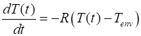
Mathematically Newton’s Law of Cooling can be written as a first order
ordinary differential equation (1) T instantaneous
temperature of the object [ oC ] t
time [ s ] R cooling
constant (depends on the thermal energy transfer mechanism, the contact area
with its surroundings and the thermal
properties of the object [
min-1 ] Tenv ambient
temperature of the surrounding environment (assumed constant) [oC
]
Newton’s Law of Cooling given
by equation 1 can be solved analytically or numerically when the
system’s initial temperature is T0.
|
||||
|
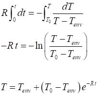
Analytical
Solution Integrate both sides of equation 1
|
||||
|
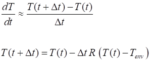
Numerical
Solution A standard technique for the numerical solution of differential
equations involves converting the differential equation into a finite
difference equation. The Euler method can be used to solve equation 1
numerically:
|
||||
|
MATLAB solutions for Newton’s Law of Cooling The function tp_fn_Newton.m can be used to solve many problems
related to Newton’s Law of Cooling. Equation 1 is solved both analytically
and numerically. Download the mscript for the function and check that you
understand the structure of the coding and how the code performs the
calculations. The function and its inputs are: function [ ] = tp_fn_Newton(R,N,tMax,T0,Tenv, flagC) % R Cooling constant
[1/min] % N Number of time steps
% tMax Time interval for simulation [minutes] % T0 Initial temperature of
system [degC] % Tenv Temperature of surrounding
environment [degc] % flagC
== 1 % Plot
numerical solution only for T vs t % flagC
== 2 % Plot of
numerical and analytical solutions for T vs t % flagC
== 3 % Plot of
numerical solution fitted to data for cooling coffee … The function is run from the
Command Window, for example tp_fn_Newton(0.05,500,60,100,0,2); is used for a simulation with the
input parameters
R = 0.05
rate constant expressed in minutes-1
N = 500
number
of time steps
tMax = 60 length of simulation
time in minutes
T0 = 100
initial temperature of system in oC
Tenv = 0
surrounding environmental temperature in oC
FlagC = 1 or 2 or 3 determines the
graphical output to be displayed. The output of the function is
displayed graphically and a summary of the input and output parameters is
shown in the Command Window as shown below: >> tp_fn_Newton(0.05,500,60,100,0,2); Cooling constant
R = 5.000e-02 [1/min] Number of time steps
N = 500 Time interval for
simulation tMax = 60 [min] Environmental temperature Tenv =
0.00 [degC] Initial temperature of
system T0 = 100.00 [degC] Final temperature of system Tend = 4.93 [degC] |
||||
|
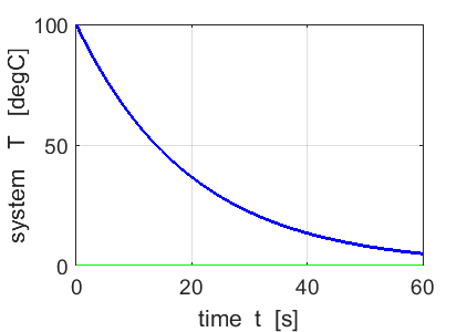
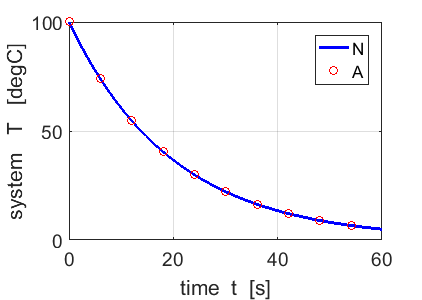
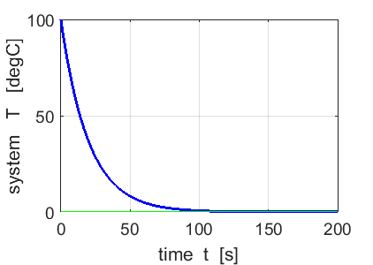
Fig.
1A. Temperature of the
system as it approaches the ambient temperature of 0 oC. |
Fig.
1B. The numerical and
analytical solution of equation 1 (N = 500). |
|||
|
For a
large number of time steps N = 500, there is excellent agreement between the
predictions of the numerical and analytical computations as shown in figure
1B. Generally, the larger the number of time steps for the numerical
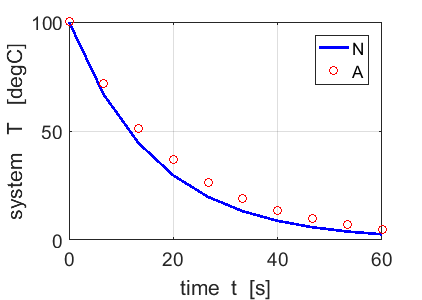
computation, the better the agreement with the analytical predictions. Figure
2 (N = 10) shows poor agreement between the numerical and analytical
predictions when a small number of time steps is used. One
should always check when using numerical methods that the step size is small
enough so that you get accurate results. You can often do this by continually
doubling the size of N (halving the step size) until there is no significant
changes in the results of the computation. |
Fig.
2. The numerical and
analytical solution of equation 1 (N = 10). |
|||
|
EXPLORATIONS ON NEWTON’S
LAW OF COOLING USING THE FUNCTION
function [ ] = tp_fn_Newton(R,N,tMax,T0,Tenv, flagC) 1. Exponential Decay 1.1 By varying the input parameter tMax, find the time it takes the system to cool from 100 oC to 0 oC
for a cooling constant
R = 0.05. 1.2 Find the times for the
temperature of the system to drop from 100 oC
to 50 oC, 25.0 oC
and 12.5 oC.
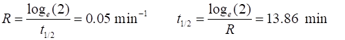
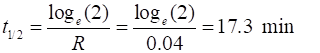
What is the effective half-life time t1/2 and
how is it related to the cooling constant R? 1.3 How long does it take for the
temperature of the system to drop from 80 oC
to 40 oC? Explain the result. |
||||
|
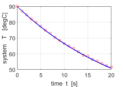
2. Coffeee Cooling Problem A hot
cup of coffee left standing will always cool down. An experiment was performed in which
the temperature of a hot cup of coffee was measured every minute for 20
minutes. The initial temperature of the coffee was 90 oC
and the ambient temperature was 20 oC.
The measurements are recorded in the mscript. Find
the cooling constant R for the hot coffee cup loosing thermal energy to its
surroundings at a constant rate. Start
with R = 0.01, N = 5000, tMax = 60, T0 = 90, Tenv = 20, flagC = 3 >> tp_fn_Newton(0.01,5000,60,90,20,3); How
well does Newton’s Law of Cooling describe the cooling of the coffee? From
the graphically output, find the value of t1/2 and calculate R.
How does your calculated value of R compare with the value of R used in the
input? It is a good idea to make your own measurments for the
cooling of the coffe and enter your data enter into the mscript. |
||||
|
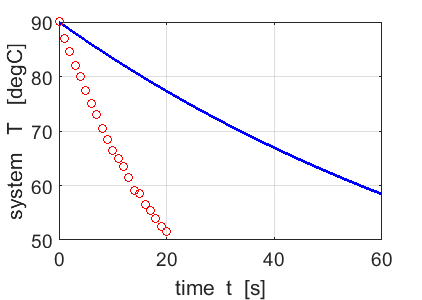
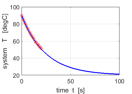
Fig. 3.
Initial attempt at fitting
the exponetial decrease in temperature to measured date for the coffee. The
red cirles show the measurements. tp_fn_Newton(0.01,5000,60,90,20,3); Change the
input parameters of the function to get the best estimate of the cooling
constant R. |
|
|||
|
3. CSI: MURDER – time of
death At the scene of a crime a
dead person was found. Can you determine the time of death? What details do you need to
know? What meaurements need to be
taken? The temperature of the body
was measured to be 32.0 oC at 5.00 pm and at 28.5 oC on
hour later at 6:00 pm. The room temeprature was 22 oC. Estimate an uncertainty in
the time of death assuming that the room temperature measurement could have
fluctuated by 1oC. |
||||
|
EXPLORATION SOLUTIONS |
||||
|
1. Exponential Decay tp_fn_Newton(0.05,5000,200,100,0,2); 1.1 Time to reach
ambient temperature ~ 120 minutes 1.2 T1 = 50 oC t1 = 13.86 min
T2 = 25 oc t2 = 27.71 min
t2 – t1 = 13.85 min
T3 = 12.5 oC t3 =
41.56 min
t3 – t1 = 13.85 min
Half-life time interval = (13.85
(measurements using Data cursor)
1.3 T1 = 80 oC t1 = 4.44 min
T2 = 40 oc t2 = 18.32 min t2
– t1 = 13.88 min
|
|
|||
|
2. Coffee Cooling Problem R =
0.04 is the best estimate. The
predictions using Newton’s Cooling Law with R = 0.04 agree very well
with the measured temperatures of the coffee. tp_fn_Newton(0.041,5000,100,90,20,3); |
||||
|
|
|
|||
|
Take
T1 = 80 oC t1 = 4.00 min T1 -Tenv = (80 – 20) oC
= 60 oC To
calculate Therefore,
|
||||
|
3. CSI: MURDER – time of
death Measurements Tenv
= (22 Tbody
= 37 oC
normal body temperature At 5:00 pm T = 32.0 oC At 6:00 pm T = 28.5 oC You
need to calculate the cooling constant R for the drop in temperature of the
victim from 32.0 oC to 28.5 oC in 60 minutes. This
is done by a trial and error process by changing the value of R using the
function tp_fn_Newton.m in the Matlab Command Window >>
tp_fn_Newton(7.18e-3,5000,60,32,22,1) returns the
following output in the Command Window Cooling
constant
R = 7.180e-03 [1/min] Number
of time steps
N = 5000 Time
interval for simulation tMax = 60 [min] Environmental
temperature
Tenv
= 22.00 [degC] Initial
temperature of system T0 = 32.00 [degC] Final
temperature of system
Tend = 28.50 [degC] >>
tp_fn_Newton(8.2e-3,5000,60,32,23,1); Cooling
constant
R = 8.200e-03 [1/min] Number
of time steps
N = 5000 Time
interval for simulation tMax = 60 [min] Environmental temperature Tenv =
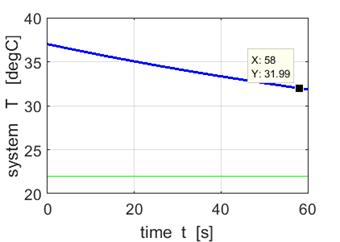
23.00 [degC] Initial temperature of system T0 = 32.00 [degC] Final temperature of system Tend = 28.50 [degC] Take
the value of R and its uncertainty to be R = (7 and
execute the function to find the time the time for the victim’s
temperature to drop from 37 oC to 32 oC |
||||
|
R =
7x10⁻³ min-1
Time
interval = 58 min |
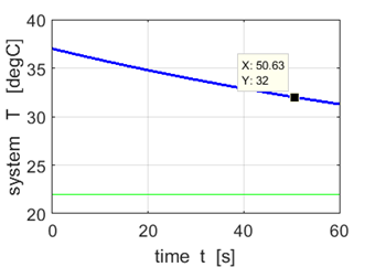
R =
8x10⁻³ min-1
Time
interval = 51 min |
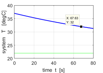
R =
6x10⁻³ min-1
Time
interval = 68 min |
||
|
Our
estimate for the time interval for the temperature of the victim to drop from
37 oC to 32 oC
is (58 Therefore,
our best estimate for the time of the murder is between 3:50 pm and 4:10 pm. |
||||