|
|
THERMAL PHYSICS SECOND LAW OF THERMODYNAMICS
Arrow
of time Ian Cooper School of Physics, University of Sydney ian.cooper@sydney.edu.au DOWNLOAD
DIRECTORY FOR MATLAB SCRIPTS tp_equilibrium.m The mscript is for a simulation of the release of
“perfume molecules” from a corner of a room and predicting how
these gas molecules will distribute themselves throughout the room. The
motion of the gas molecules can be saved as an animated gif. SECOND LAW OF THERMODYNAMICS The Second
Law of Thermodynamics can be
stated as: Natural process in an isolated system
will always spontaneously evolve to states of greater disorder (states of
greater entropy – states of greater probability) We can think of the concept of entropy as a measure of the disorder of a system. But what do these statements mean? We will consider the act of releasing a small quantity of perfume into
a fully closed room from one location within the room. Immediately after the
perfume is released, we can conclude that the perfume molecules are in an orderly
state (state with the lowest entropy) since all the molecules are
located within a small volume element of the room. After some time interval, we know that
the perfume can be detected through the room and the perfume molecules will
be uniformly spread around the room. This is the most disordered state (state of maximum
entropy state of maximum probability). If we continuously
monitor the motion of all the perfume molecules we will never detect all the
molecules again located in the small volume element that they were released
from, although in terms of the principles of conservation of energy and
momentum this state is not forbidden.
Why? Because if all the perfume molecules were suddenly found within
the initial volume element it would be a violation of the Second Law of
Thermodynamics. We can help clarify the meaning of order / disorder and entropy by
using a simple model to account for the behavior of the perfume gas molecules.
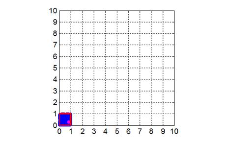
We will consider the gas to be enclosed within an area A = 10x10
a.u., that is, we will consider the
behavior of N gas molecules from a
two-dimensional point of view. The enclosure is divided into 100 equal size
boxes of area Abox
= 1x1 a.u. At time t = 0 all the gas molecules are within the box
(outlined in red) located near the origin (0,
0) as shown in figure 1.
Fig. 1. The
two-dimensional enclosure of the gas with an area A = 10x10 a.u. The area is subdivided
into 100 boxes of area Abox = 1x1 a.u. At time t
= 0, all the gas molecules (N =
600) are released from the
box outlined in red.
One of the gas molecules is marked so that you can track its movements. tp_equilibrium.m The initial state of the gas at t
= 0 has the most order since the molecules are located into the smallest
volume element and there is only one arrangement possible for this as all the
molecules are in one of the boxes. After the gas is released, each molecule
moves a random distance and direction in each time step. We are interested in
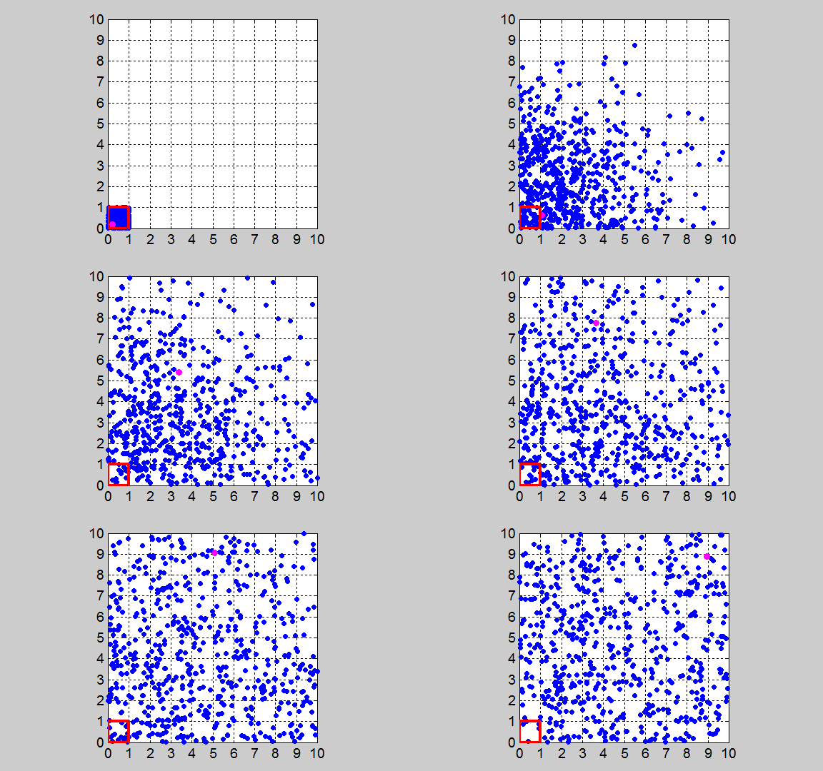
how the molecules arrange themselves in the 100 boxes as time flows. The
movement of the gas molecules is shown in the animation of figure 2.
Fig. 2. Animation of
gas molecules released from the red enclosed box at time t = 0. The distribution of the gas molecules evolves to states that are more
probable. This means the gas molecules after being released will eventually
fill uniformly the entire enclosure. The system evolves with time to the
state which has its maximum entropy and this corresponds to the most probable
state. The system evolves to an
equilibrium state in which each box has the same number of molecules in it
since this is the state in which there is the greatest number of ways in
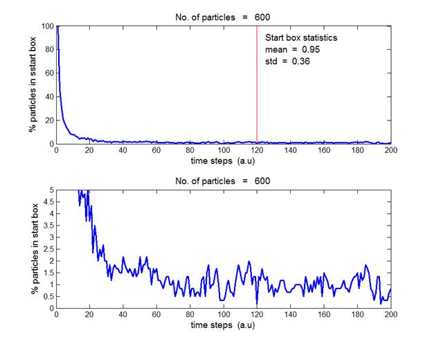
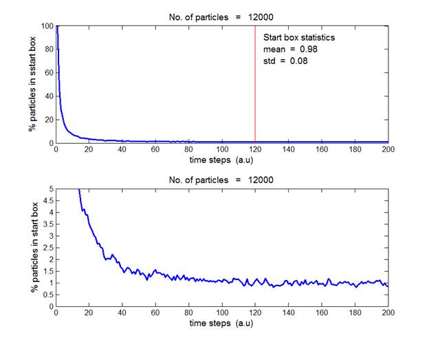
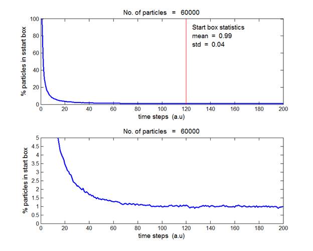
which the gas molecules can arrange themselves in the 100 boxes. Figures 3, 4 and 5 ( tp_equilibrium.m ) show the percentage of the gas
molecules in the red box (unit area Abox
= 1x1 a.u.) – the box from which the N particles were released from. Since there are 100 boxes, in the
equilibrium state (state with the maximum number of ways the particles can
arrange themselves à the most probable state à state with the maximum entropy) has 1.00 % of
the total N particles in the start box. The mean and standard deviation for the
average percentage of particles in the start box in the time interval from t = 120 to 200 a.u.
are shown in each figure. The standard deviation means that in 68% of the
measured time steps, the percentage was within one standard deviation of the
mean. In each figure, the bottom
view shows the y-axis scale reduced to 0 to 5% for the particles in the start
box.
Fig. 3. N = 600 gas molecules. The average
percentage of particles in the starting box in the time interval
from t
= 120 to 200 a.u. is (0.93 ± 0.36).
Fig. 4. N = 12 000 gas molecules. The average
percentage of particles in the start box in the time interval
from t
= 120 to 200 a.u. is (0.98 ± 0.08).
Fig. 4. N = 60 000 gas molecules. The average
percentage of particles in the start box in the time interval from t = 120 to
200 a.u. is
(0.99 ± 0.04). Inspection of figures 3, 4 and 5 show that as the number of particles
increase, the mean value approaches 1% and its uncertainty becomes smaller.
It is clear that as N gets larger,
the distribution becomes more uniform and the fluctuations from the mean value
reduce. 60 000 particles was the maximum number of particles used in the
three simulations. Consider a gas enclosed in a volume V = 1.00 m3 at atmospheric pressure p = 1.01x10⁵ Pa and
temperature T = 300 K. In this
volume there are 2.4x1025 particles ( p V = N
k T ). In a box of 1.00 m3, the gas molecules
will certainly be uniformly distribution and the any fluctuations away from
this equilibrium state will certainly be negligible. Hence, the process of
the gas spreading around the room is irreversible. Although it is possible that
all the particles can return to the start box at the same instant, there are
no laws really preventing this, only that the probability of this occurring
is exceedingly small. When the perfume is released, the system of the enclosed gas
spontaneously changes from a state of low probability to one of higher
probability, that is, the entropy of the system increases. The relationship
between probability and entropy is given by
S = k loge( w ) where S is the entropy, k is the Boltzmann constant and w is “loosely” defined as the number of molecular
arrangements that correspond to the same macroscopic state. In our initial
state (t = 0), there is only one
possible arrangement of the particles – all the particles must be in
the start box, w = 1 à S = 0. The Second
Law of Thermodynamics, tells us that if an isolated system
undergoes a spontaneous process, its final state will be one in which the
entropy S and w are maximum. MATLAB MSCRIPT Setup for initial position of particles in start box using the Matlab
command rand to give a set of
numbers between zero and one e.g. rand(1,5) à 0.7612 0.7568 0.3738 0.5126 0.9739 % initial position of N
particles within unit box ------------------------
R = 1;
% max step
length
P = rand(N,2);
% initial (x,y) coordinates of N particles
x = P(:,1);
y = P(:,2); Particle coordinates are updated in a for loop using the Matlab
command randn
to give random numbers which are normally
e.g. randn(1,5) à -0.0426 0.8961 -2.1927 -1.3408 0.0100 % increment the position of each
particle --------------------------------
dP = R.*randn(N,2);
dx = dP(:,1);
dy = dP(:,2);
% updated position of each
particle---------------------------------------
x = x + dx;
y = y + dy; The particles are kept inside the enclose by reflections at the sides % particle reflected of
boundaries of the box ---------------------------- for c1 = 1:N if x(c1) < 0; x(c1) = x(c1) +
abs(dx(c1)); end; if y(c1) < 0; y(c1) = y(c1) + abs(dy(c1));
end; if x(c1) > 10; x(c1) = x(c1) -
abs(dx(c1)); end; if y(c1) > 10; y(c1) = y(c1) - abs(dy(c1)); end;
end To count the number of particles in the start box each time step,
logical functions are used e.g. z = rand(1,5) à
0.7635
0.0078
0.8026 0.7228 0.7291 0.0627 0.7569 0.6265 0.1902 .6564
z01 = z01 < 0.5 à 0
1
0
0
0
1
0
0
1
0
z10 = z(z<0.5) à 0.0078 0.0627 0.1902
sum of numbers less than 0.5 sum(z01) à 3 % calculate the number of particles in
start box -------------------------- box_x = ones(1,N); box_y = ones(1,N); box_x(x>R) = 0; box_y(y>R) = 0; N_box(c) = sum(box_x .* box_y); Calculating the statistics for the start box
% calc. mean std sem
for no. of particles in start box ---------------
ns = floor(0.6*nt);
% starting point
for calc.
N_avg = (100/N) * mean(N_box(ns:end));
N_std = (100/N) * std(N_box(ns:end));
N_sem = N_std/sqrt(nt-ns+1); |
