|
Ian Cooper matlabvisualphysics@gmail.com WAVE MOTION FREQUENCY SPECTRUM OF AN EXCITED STRING THE WAVE EQUATION AND FOURIER TRANSFORM DOWNLOAD
DIRECTORIES FOR MATLAB SCRIPTS em_swe_01A.m The [1D] wave equation
can be solved numerically using a finite difference method for the vibrations
of a string with given boundary conditions
where The string is initially
excited by random fluctuations along its length. The string can also be
clamped at any point xc The Script em_swe_01A.m is used to
solve the wave equation for the transverse displacement function Input: % Number of spatial grid points Nx
= 201; % Number of time steps Nt
= 2201; % length of simulation
region L = 10; % wave or propagation speed v = 20; % Courant number S = 1; % Thee signal detection location SL / Clamped string
location CL (indices)
SL = round([Nx/2, Nx/3,Nx/4]); CL = round([Nx/3 2*Nx/3]); % CL = 1; Setup: % Spatial grid spacing / time step / spatial grid hx
= L / Nx; ht
= S * hx / v; S2 = S^2; x = linspace(0,
L , Nx); t = linspace(0,ht*Nt,Nt); % Random initial conditions (comment / uncomment rand
# selection u = zeros(Nx,Nt); % u(2:Nx-1,1)
= 0.25.*rand(Nx-2,1); u(2:Nx-1,1) = 1 .* (2.*rand(Nx-2,1) - 1); Finite Difference Time
Development Method – solving the wave equation: for nt = 2 :
Nt-1 for nx = 2 : Nx-1 u(nx,nt+1) = 2*u(nx,nt)-
u(nx,nt-1)+ S2*(u(nx+1,nt) - 2*u(nx,nt) +
u(nx-1,nt)); % Clamped location (comment / uncomment u(CL,nt+1) = 0; end % Boundary Conditions comment / uncomment u(1,
nt+1) = 0;
% Fixed end u(Nx, nt+1) = 0;
% Fixed end end FOURIER
TRANSFORM % Frequency range fMax
= 10; f = linspace(0,fMax,Nt); % Initialize F.T. %
HB = zeros(1,Nt); HR =
zeros(1,Nt); HM = zeros(1,Nt); HB = FT(u(SL(1),:),f,t,Nt); psdB
= HB.*conj(HB); HR = FT(u(SL(2),:),f,t,Nt); psdR
= HR.*conj(HR); HM = FT(u(SL(3),:),f,t,Nt); psdM
= HM.*conj(HM); function H =
FT(u1,f,t,Nt) H = zeros(Nt,1); %
Fourier Transform H(f) for
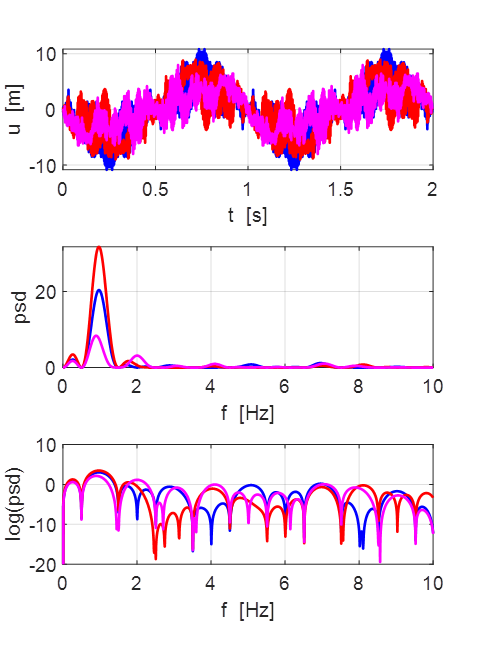
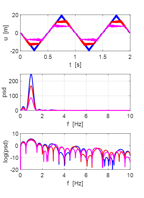
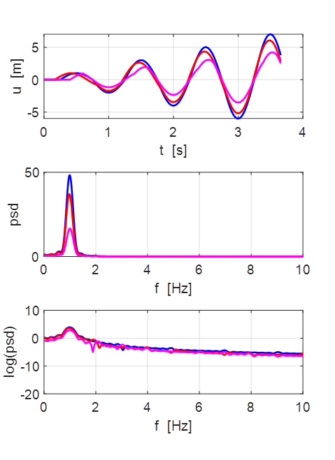
c = 1:Nt g = u1 .* exp(1i*2*pi*f(c)*t); H(c) = simpson1d(g,min(t),max(t)); end SAMPLE RESULTS L = 10 m v = 20 m.s-1 fundamental: f = 1.00 Hz T = 1.00 s String only clamped at its end
Transverse
displacement of string
(u(2:Nx-1,1) = 1 .* (2.*rand(Nx-2,1) - 1);)
Oscillations at x = L/2 (blue), x = L/3 (red) and x =
L/4 (magenta).
All three points oscillate with the predominant frequency component
equal to the
fundamental frequency of 1.00 Hz. The oscillations are not sinusoidal.
(u(2:Nx-1,1) = 1 .* (2.*rand(Nx-2,1) - 1);)
Transverse
displacement of string u(2:Nx-1,1) = 0.25.*rand(Nx-2,1);
Oscillations at x = L/2 (blue), x = L/3 (red) and x =
L/4 (magenta).
All three points oscillate with the predominant frequency component
equal to the fundamental
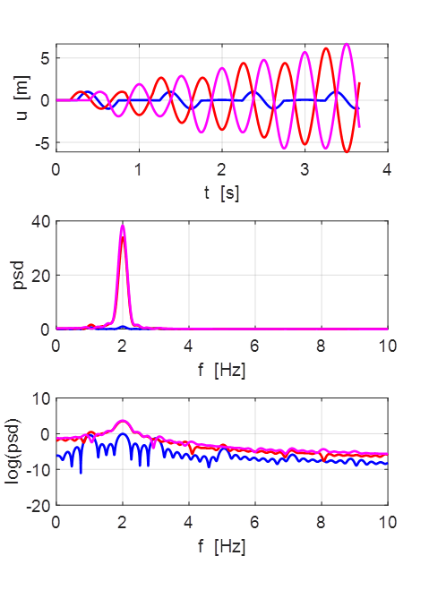
frequency of 1.00 Hz. The oscillations are not sinusoidal. u(2:Nx-1,1) = 0.25.*rand(Nx-2,1); String clamped at x = L/2
Transverse displacement of string
(u(2:Nx-1,1) = 1 .* (2.*rand(Nx-2,1) - 1);)
Oscillations at x = L/2 (blue), x = L/3
(red) and x = L/4 (magenta).
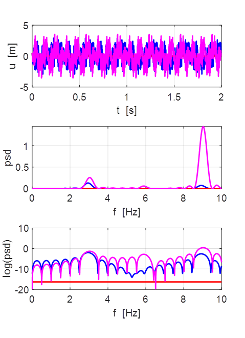
At x = L/2 there is a node since the string is clamped at this
position.
The even harmonics are mainly excited with the peak in the spectrum
occurring at the frequency of the 2rd harmonics.
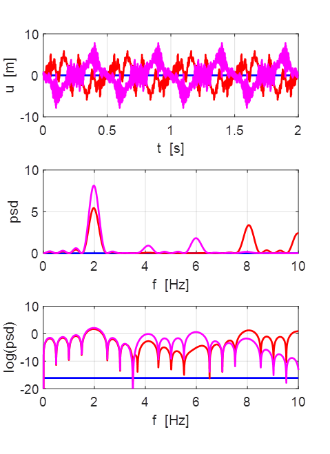
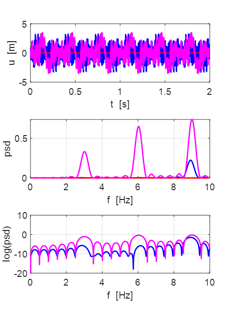
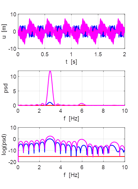
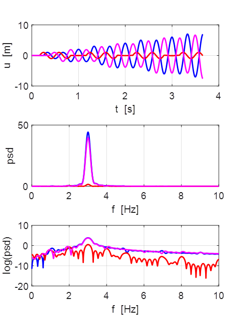
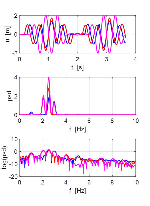
(u(2:Nx-1,1) = 1 .* (2.*rand(Nx-2,1) - 1);) String clamped at x = L/3 and x = 2L/3
Transverse displacement of string
(u(2:Nx-1,1) = 1 .* (2.*rand(Nx-2,1) - 1);)
Oscillations at x = L/2 (blue), x = L/3 (red) and x =
L/4 (magenta).
At x = L/3 there is a node since the string is clamped at this
position.
The other two points oscillate almost at the frequency of the 3rd
harmonics.
The main frequency
components excited ate the harmonics 3, 6, 9. Each time
The Script is run, the distribution of energy into the harmonics 3, 6,
9 is different.
(u(2:Nx-1,1) = 1 .* (2.*rand(Nx-2,1) - 1);) Natural frequencies of oscillation: Driven string The Script can be modified
by commenting and uncommenting the code to excite the string at x = 0 by
a sinusoidal signal with frequency f0. for
nt = 2 :
Nt-1 for
nx = 2 : Nx-1 %
sinusoidal excited at x = 0; u(1,nt+1) = 1*sin(2*pi*f0*t(nt)); u(nx,nt+1) = 2*u(nx,nt)- u(nx,nt-1)+
S2*(u(nx+1,nt) - 2*u(nx,nt) + u(nx-1,nt)); %
Clamped location
(comment / uncomment % u(CL,nt+1) = 0; end %
Boundary Conditions
comment / uncomment % u(1, nt) = 0;
% Fixed end u(Nx, nt)
= 0; % Fixed end end Fundamental 1st
harmonics f0
=1
Second harmonic f0 = 2
Third harmonics f0 = 3
Non-harmonic frequency f0 =
2.5
|