|
HELMHOLTZ EQUATION EIGENVALUE PROBLEM TRANSVERSE STANDING
WAVES ON A ROD Ian
Cooper Email: matlabvisualphysics@gmail.com wm_Helmholtz.m Solution of the Helmholtz
equation for the transverse vibrations of a rod with boundary conditions that
can be either fixed or free. The modes of vibration of the rod are found by
finding the eigenvalues and corresponding eigenfunctions for the Helmholtz
equation expressed in matrix form. The INPUT section of the Script is used to
enter the boundary conditions, number of time steps, number of spatial grid
points, the length of the rod, the transverse wave velocity and the mode of
vibration for the standing wave. The animated motion can be saved as an
animated gif file by setting flagS = 1. The script
could be altered so the animation could be saved as an avi
file and the input parameters entered via the Command Window or using the
Live Editor. Link to
Script https://github.com/D-Arora/Doing-Physics-With-Matlab/blob/master/mpScripts/wm_Helmholtz.m THE
HELMHOLTZ EQUATION The Helmholtz equation is (1) where The Helmholtz equation
represents a time-independent form of the wave equation and results from
applying the technique of separation of variables to reduce the complexity of
the analysis. (2) It is often convenient to assume that the
wavefunction (3) By substitution of equation 3 into equation 2, we can derive the Helmholtz equation (1) The [1D] form of the
Helmholtz equation is (4) The solution of the
Helmholtz equation depends upon the boundary conditions applied to the
system. STANDING
TRANSVERSE WAVES OF A ROD The motion of oscillating
systems is a classic problem in eigenvalue theory
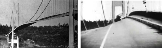
which we can easily investigate using Matlab. For example, we can
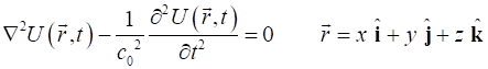
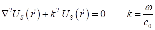
model the complex oscillations of the Tacoma Narrows Bridge in which the deck
of the bridge undergoes two kinds of vibration: one along its length and the
other from side-to-side.
Fig. 1. Vibrations along the length of the
bridge. Boundary conditions: fixed / fixed (nodes at the ends of the bridge
span).
Fig. 2. Side-to-side
vibrations. Boundary conditions: free / free (antinodes along the side of the
bridge span). We can approximate the second
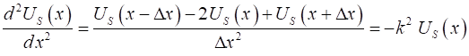
derivative by the finite difference approximation to give (5) Let the X-domain be
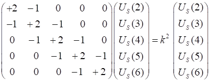
divided into For example, if N
= 5 and the boundary conditions at the ends are (6) since
. . .
We now have a simple eigenvalue problem of the form
where We are now able to solve equation 6 using the following Matlab code % Eigenvalue Matrix A: eigenfunctions (eignFN) / eigenvalues (eignV) off = ones(N-1,1); A = 2*eye(N) - diag(off,1) - diag(off,-1); [eignFN,
eignV] = eig(A); % Spatial Wavefunction US for mode m US = zeros(N+2,1); US(2:N+1)
= eignFN(:,m); US = US
./max(US); The length of
the rod is % Spatial domian [m] x = (0:N+1).*(L/(N+1)); k is the propagation constant and it needs to be scaled to express its value in rad.s-1. % propagation constant [1/m] k = sqrt(eignV(m,m))
.* (N+1)/L; The value of the
propagation constant k and
the transverse wave speed v are
used to calculate the wavelength %
angular frequency
[rad/s] w = v*k; % period [s] T = 2*pi/w; % frequency [Hz] f = 1/T; % time [s] t = linspace(0,2*T,nT); % wavelength [m] lambda =
2*pi/k; % time dependent wavefunction UT =
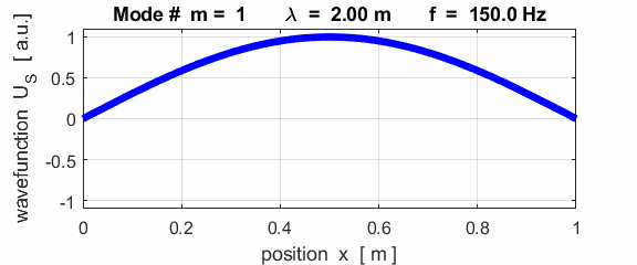
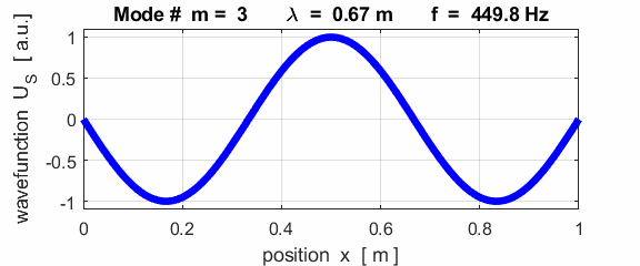
cos(w.*t); To examine different modes of vibration, the
Script is run with different values of the mode number m. So far, we have only considered nodes at each end of the rod. We can also model the vibrations of the rod with an antinode at the ends (free). Equation 5 can be written as
Antinode (free) at left end of
rod
Therefore, in the matrix A element A(1,1) = 1. Antinode (free) at the right end
of the rod
Therefore, in the matrix A element A(N+1,N+1) = 1. In the Script, the boundary conditions are set by the variable BC % Boundary conditions: fixed fixed
BC = 1 / fixed free BC = 2 / free free BC = 1 BC = 1; if BC == 2;
A(N,N) = 1; end
% fixed free if BC == 3;
A(1,1) = 1; A(N,N) = 1; end % free free if BC == 2;
US(N+2) = US(N+1); end if BC == 3;
US(1)
= US(2); US(N+2) = US(N+1); end Note: The matrix A does not include the end grid points related to the X-domain, but only the N interior grid points. Boundary conditions: nodes at
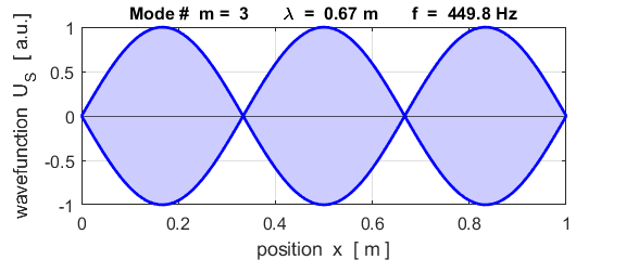
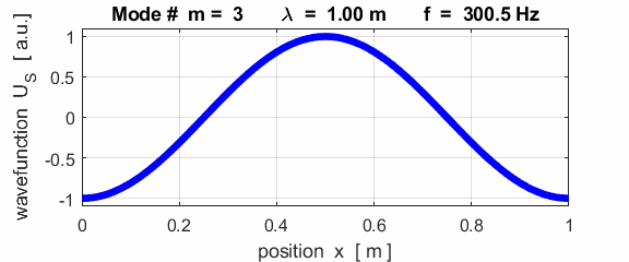
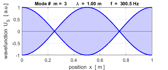
each end of the rod (fixed / fixed)
This mode of vibration is like the oscillations of the Tacoma Bridge span along its length (figure 1).
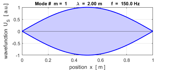
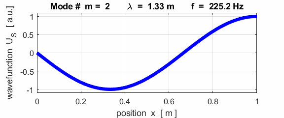
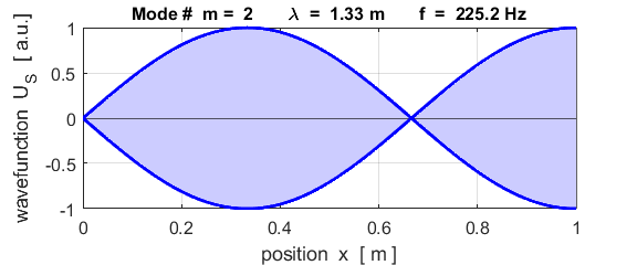
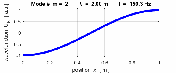
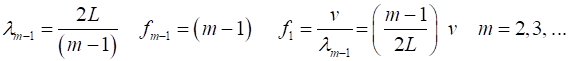
The mode m = 1 is called the fundamental or 1st harmonic mode of vibration. For the rod fixed at both ends (nodes at each end), the results of the simulations show that
where For the rod fixed at both end, all the harmonics can be excited. Note: The
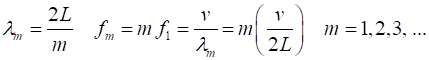
wavelength Boundary conditions: node at
left and an antinode at the right end (fixed / fixed) BC = 2
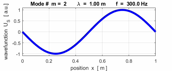
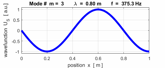
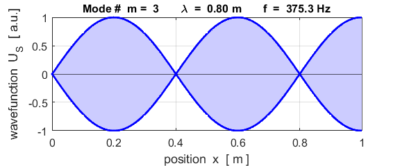
For the rod with a node at the left end and an antinode at the right end (fixed / free), the results of the simulations show that
For the rod with
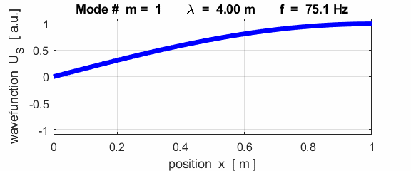
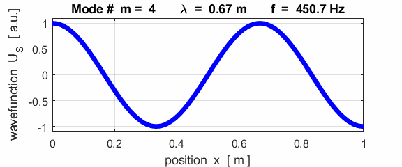
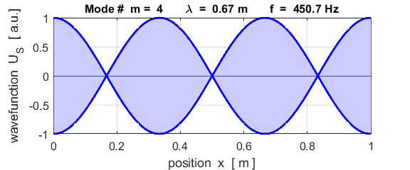
the fixed / free boundary conditions, only the odd harmonics Boundary conditions: antinode at both ends (fixed / fixed) BC = 3 (m>1)
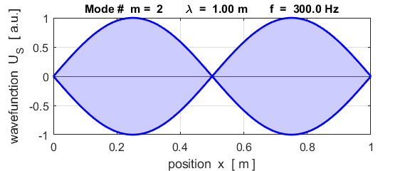
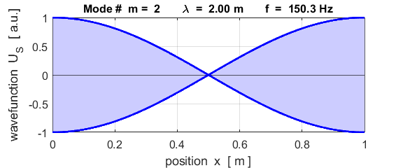
This mode of vibration is like the side-to-side oscillations of the Tacoma Narrows Bridge (figure 2).
For the rod with an antinodes at both ends of the rod (free / free), the results of the simulations show that
For the rod with
the free / free boundary conditions, all the harmonics
The Script wm_Helmholtz.m can be easily modified to model the vibrations of air columns in tubes or standing electromagnetic waves. The same equation and solution procedure is exactly the same for many very different physical situations involving standing waves. |
|
|