|
HELMHOLTZ EQUATION EINGENVALUE
PROBLEM: A VIBRATING MEMBRANE DOWNLOAD DIRECTORY FOR MATLAB SCRIPTS wm_Helmholtz2D.m Solution of the Helmholtz equation to model the
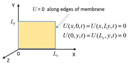
vibrations of a rectangular membrane which has a node around its perimeter.
The modes of vibration of the membrane are found by finding the eigenvalues
and corresponding eigenfunctions for the Helmholtz equation expressed in
matrix form. The INPUT section of the Script is used to enter the number of
time steps, number of spatial grid points, the dimensions of the membrane, the
transverse wave velocity and the mode of vibration for the standing wave. The
animated motion can be saved as an animated gif file by setting flagS = 1. The Script could be altered so the animation
could be saved as an avi file and the input
parameters entered via the Command Window or using the Live Editor. THE HELMHOLTZ
EQUATION Let’s consider a two-dimensional example of
the standing waves in an elastic membrane. If the rest position for the
membrane is the X-Y plane, so when it’s vibrating it’s moving up
and down in the Z-direction. The shape of the surface at any instant of time
is a function is given by the wavefunction
Fig. 1. Geometry for the vibrating
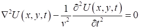
membrane. The
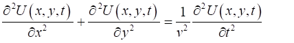
wavefunction must satisfy the [2D] wave equation (1A) (1B) To solve the wave equation 1B, we can use the method
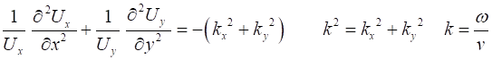
of separation of variables where solutions have the form (2) Substituting equation 2 into 1B and dividing the result by
The functions of x and y must be independent, therefore
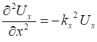
(3A)
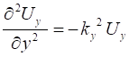
(3B) Equation 3 is the Helmholtz
equation and represents a
time-independent form of the wave equation. STANDING TRANSVERSE WAVES OF A VIBRATING MEMBRANE The motion of
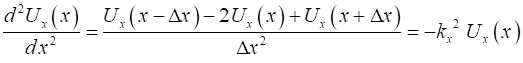
oscillating systems is a classic problem in eigenvalue theory which we can easily investigate using Matlab. For the X domain, we
can approximate the second derivative by the finite difference approximation
to give (4) Let the X-domain be
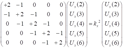
divided into For example, if N =
5 and the boundary conditions at the ends are
(5)
since
. . .
We now have a simple eigenvalue problem of the form
where For the Y domain, the
procedure is identical as given above for the X domain. We are now able to solve equation 5 using the following Matlab code
and calculate the natural frequencies of vibration for the normal modes
specified by the integers mX
and mY. % CALCULATIONS
====================================================== % Spatial domian [m] x = (0:N+1).*(LX/(N+1)); y = (0:N+1).*(LY/(N+1)); % Eigenvalue Matrix A: eigenfunctions
(eignFN) / eigenvalues (eignV)
off = ones(N-1,1); A = 2*eye(N) - diag(off,1) - diag(off,-1); [eignFN,
eignV] = eig(A); % Spatial Wavefunction US USX = zeros(N+2,1); USX(2:N+1) = eignFN(:,mX); USX = USX ./max(USX); USY = zeros(N+2,1); USY(2:N+1)
= eignFN(:,mY); USY = USY ./max(USY); USXX
= meshgrid(USX); USYY
= meshgrid(USY)'; USS = USXX.*USYY; % Time dependent wavefunction UT %
propagation constant [1/m] kX = sqrt(eignV(mX,mX)) .* (N+1)/LX; kY = sqrt(eignV(mY,mY)) .* (N+1)/LY; k = sqrt(kX^2
+ kY^2); %
angular frequency [rad/s] w = v*k; %
period [s] T = 2*pi/w; %
frequency [Hz] f = 1/T; %
time [s] t = linspace(0,1*T,nT); %
wavelength [m] lambda =
2*pi/k; % time
dependent wavefunction UT =
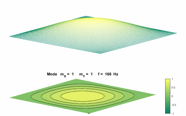
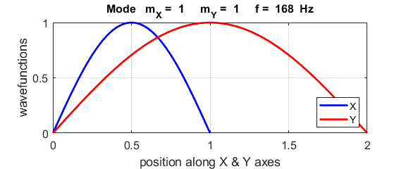
cos(w.*t); Fundamental normal mode of vibration mX = 1
mY = 1
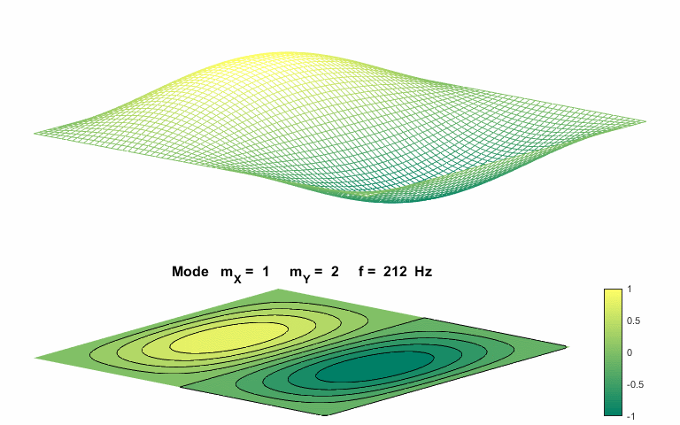
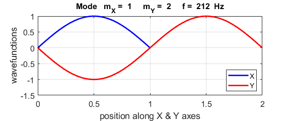
Normal mode of vibration mX =
1 mY
= 2
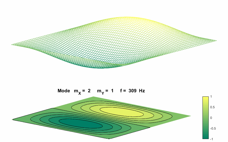
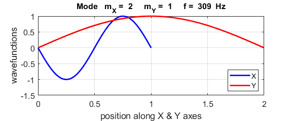
Normal mode of vibration mX
= 2 mY = 1
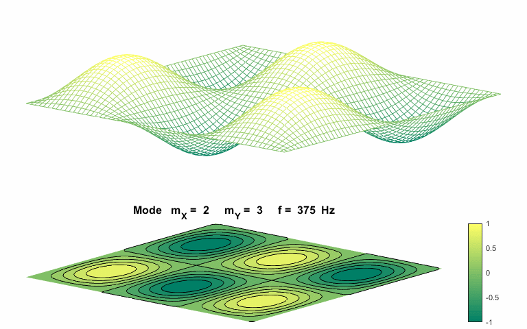
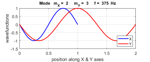
Normal mode of vibration mX =
2 mY
= 3
The natural
frequencies of vibration for a rectangular membrane do not form a harmonic
integer series. The patterns show nodal lines separating antinodal
regions. |
|
Ian Cooper matlabvisualphysics@gmail.com |