|
PROPAGATION OF WAVEFORMS
To
illustrate the properties of travelling or progressive waves, we will
consider the propagation of transverse disturbances on strings. This is
easy to treat mathematically and the results are applicable to
electromagnetic waves, sound, matter waves and other types of waves.
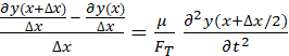
Consider
a uniform string of linear density  stretched along the X-axis under a
tension FT
. The disturbance of the string is confined
to the XY-plane. The displacement of the string y
is transverse to the direction of propagation of the waveform and is
assumed to be small and any bowing of the string due to its weight is
neglected. The disturbance along the string y
is determined by the one-dimensional wave equation stretched along the X-axis under a
tension FT
. The disturbance of the string is confined
to the XY-plane. The displacement of the string y
is transverse to the direction of propagation of the waveform and is
assumed to be small and any bowing of the string due to its weight is
neglected. The disturbance along the string y
is determined by the one-dimensional wave equation
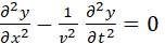
(1)
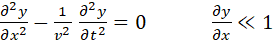
where
v
is the speed of the waveform along the string and is given by the equation
(2)

Eq.
(1) is a linear second order partial differential equation. Because of its
linearity, if the wavefunctions y1
and y2
are both solutions that satisfy Eq. (1) then their sum y1
+ y2
is also a solution (Superposition Principle). The quantity  is a measure of the strings curvature at any instant and therefore, of the
string tension. The quantity is a measure of the strings curvature at any instant and therefore, of the
string tension. The quantity  is proportional
to the acceleration of a small segment of the string. is proportional
to the acceleration of a small segment of the string.
The
speed v
depends only on the values of FT
and .
The only way to increase the propagation speed is to increase the string
tension or use a string with a smaller value for its linear density.
Derivation Eq. (2)
– speed of a transverse wave on a string
A
simple model is used to determine the speed of propagation v of a transverse wave
along a stretched spring. One end of the cord is pulled upward by a force Fy
with a speed vy.
In a time t,
the string is lifted as a straight segment so that the displacement of the
end of the string is vy t
and the pulse travels along the string with a speed v and the leading end of
the pulse travels a distance v t. We assume that the vertical
displacement of the string is small ( is small or is small or  ). ).
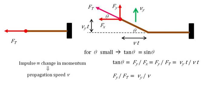
Fig.
1. The end of the string is
pulled upward by a force Fy
with a speed vy. The pulse travels along the string
at a speed v.
We assume that the end of the string is lifted as a straight segment with
the angle being small.
In
the time t,
the vertical impulse produces a change in momentum of the segment of the
string that is lifted
 QED QED
Derivation Eq. (1)
– [1D] wave equation
A
simple model is used to derive the [1D] wave equation describing the
propagation of transverse waves along strings. It is assumed that the
deflection of the string is small ().
The derivation is based upon the application of Newton’s Second Law
to a small segment of the string of mass  . .
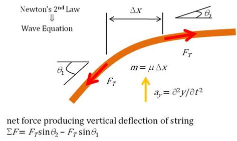
Fig.
2. A net vertical force acting
on a segment of the string causes the segment to be deflected with an
acceleration ay.

Since
is small 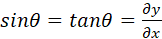
hence
In
the limit as 
 QED QED
Wave Equation Solutions
The
general solution of the wave equation, Eq.(1) is
of the form
(3) 
where
the functions f and g
have well defined second derivatives. The function f
describes a disturbance moving with speed v
in the +X direction with no change in shape or size of the disturbance and g
describes an undistorted disturbance travelling with speed v
in the –X direction. To prove this statement about f,
consider the waveform at time t and time  and at positions x
and and at positions x
and 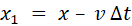
(4)

This
means that the value of the function f at
the position x and time has the same value as it was at time t
but at the position that lies to the left of x
by a distance  .
Hence, the waveform moves to the right with a speed v.
The same argument shows that the function g represents
the waveform moving to the left with a speed v. This
is the essence of wave motion. For the wave moving in the +X direction,
whatever one sees at a point x,
one sees in the same form at a point .
Hence, the waveform moves to the right with a speed v.
The same argument shows that the function g represents
the waveform moving to the left with a speed v. This
is the essence of wave motion. For the wave moving in the +X direction,
whatever one sees at a point x,
one sees in the same form at a point  but a time but a time  later, where later, where  . .
The
exact form of the functions f and g is
immaterial, all that matters is that y
is expressed in terms of (v t ± x). For
example, consider the pulse which moves to the right
(5)
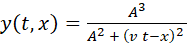
Fig.
(3) shows an animation of the pulse described by Eq. (5).
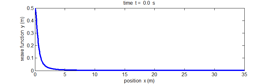
Fig.
3. An animation of the pulse
given by Eq. (5) for the time interval 0 to 10 s. The string tension is FT
= 9.0 N and linear density of the string is m
= 1.0 kg.m-1. This gives the propagation speed of the pulse as v
= 3.0 m.s-1. The pulse parameter is A
= 0.5 m. The peak of the pulse takes 10 s to move from position x
= 0 to x
= 30 m, hence the velocity as expected is 3.0 m.s-1. Matlab
script: ag_pulse1.m.
Animated gif: ag_pulse1.gif.
For
a waveform to satisfy the wave equation, Eq. (1), the condition ()
must be satisfied. This condition can be easily verified using a Matlab
script for the waveform by using the command gradient. The
waveform defined in Fig. (3) does satisfy this gradient condition as illustrated
in Fig. (4).
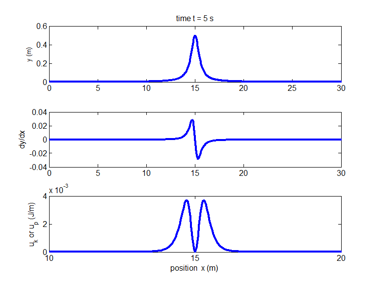
Fig.
4. Plots of
the displacement and its gradient for pulse described in Fig. (3) at time t
= 5.0 s and a plot of the energy density function for the potential and
kinetic energies up
and uk . The
maximum value of the gradient is  as required for the equation of the
pulse to satisfy the wave equation. Matlab script: ag_pulse1.m as required for the equation of the
pulse to satisfy the wave equation. Matlab script: ag_pulse1.m
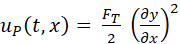
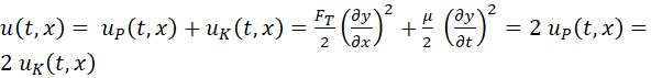
ENERGY IN A WAVE
Wave
motion is the mechanism where energy is transferred from the source through
the surrounding medium. At any instant the particles of the medium carrying
a wave are in various states of tension and motion. The medium is endowed
with energy in the form of potential and kinetic energy. The potential
energy density (energy / length) can be calculated from the work required
to stretch the string the required amount. The portion of the string
between x
and  is
stretched to a length is
stretched to a length  .
The work required to stretch the string this amount is .
The work required to stretch the string this amount is

where
the assumption that  and
the binomial expansion are used. and
the binomial expansion are used.
In
the limit as  ,
the work done per unit length becomes the potential energy density ,
the work done per unit length becomes the potential energy density
(6)
The
kinetic energy of a mass 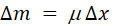 moving
with a transverse velocity moving
with a transverse velocity 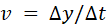 is is 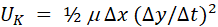 ,
hence, kinetic energy density is ,
hence, kinetic energy density is
(7)
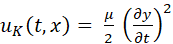
We
have  and and  ,
hence, uk = up i.e. the potential energy and the kinetic energies are
equal. A graph of the energy density functions up
and uk
at the time t
= 5.0 s are shown in Fig. (4). ,
hence, uk = up i.e. the potential energy and the kinetic energies are
equal. A graph of the energy density functions up
and uk
at the time t
= 5.0 s are shown in Fig. (4).
The
total energy density u
is
(8)
Energy
is transferred along the string and this can be described by the energy
flux S(t, x)
which is defined to be the net energy U(t, x) transferred past the
point x
per unit time. The net inflow of energy into a segment must be equal to the
rate of increase of the total energy in that segment of the string.

(9)
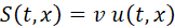
The
energy flux or power transferred  is proportional to the speed of
propagation and the total energy density. The propagation of energy by the
wave is shown by the animation of Fig. (5). Energy is transferred in the
form of kinetic and potential energy from one segment of the string to the
next while the string itself is deflected not in the direction of
propagation but at right angles to it. is proportional to the speed of
propagation and the total energy density. The propagation of energy by the
wave is shown by the animation of Fig. (5). Energy is transferred in the
form of kinetic and potential energy from one segment of the string to the
next while the string itself is deflected not in the direction of
propagation but at right angles to it.
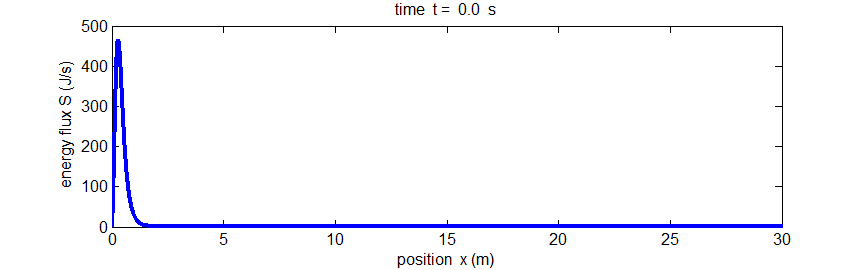
Fig.
5. The propagation of energy along the string by the pulse given by Eq.(5). The energy flux S(x,t)
is the rate at which energy passes the point x.
Matlab script: ag_pulse1.m. Animated
gif: ag_pulseE.gif.
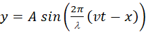
TRAVELLING SINUSOIDAL WAVES (HARMONICS WAVES)
The
most important type of travelling wave is a sinusoidal
travelling wave or harmonic wave
since other types of waves can be constructed by the superposition of
harmonics waves. The transverse displacement y(t,x) of
the string which is a function of (v t
– x) and satisfies the wave equation for
a wave propagating in the +X direction is given by Eq. (10)
(10)
A
harmonic wave travelling in the –X direction is 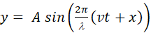 .
The maximum value of y
is known as the amplitude A.
The quantity .
The maximum value of y
is known as the amplitude A.
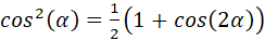
The quantity  is called the phase of the wave and is measured in radians. For one cycle of
a sine curve the phase changes by is called the phase of the wave and is measured in radians. For one cycle of
a sine curve the phase changes by  radians since radians since  .
The wave repeats itself every wavelength .
The wave repeats itself every wavelength  ,
for example at ,
for example at 
By
similar arguments, the wave also repeats in a time T called the period where and the reciprocal of the period is
known as the frequency f. The frequency is the number of
cycles per unit time.
Hence
the phase speed of the wave is  . .
The
angular frequency is  and the angular wave number (spatial frequency
or propagation constant) is and the angular wave number (spatial frequency
or propagation constant) is  . .
Therefore,
the wave shape given by Eq. (10) can also be written as
(11)

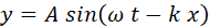
If
we took a series of picture of the wave, then at each instant, the shape of
the wave in space is sinusoidal as shown in Fig. (6) which shows an
animation of a travelling sinusoidal wave that is updated each second.
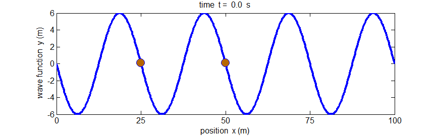
Fig.
6. A travelling sinusoidal wave. The period of the wave is 20 s and the
wavelength is 25 m. The waveform moves to the right one wavelength in a
time of one period. The circles show that each point along the wave
executes SHM. The phase speed of the wave is 1.25
m.s-1. Matlab script: ag_sine1.m. Animated gif: ag_sine1.gif.
If
we consider a fixed point, x
= x1,
then the displacement of the string at this point corresponds to simple
harmonic motion
 where
where  is a constant is a constant
For
a sinusoidal wave, each point along the string is oscillating with simple
harmonic motion with a period T
and points separated by a distance equal to one wavelength are oscillating in phase with each
other as shown in Fig. (6).
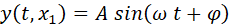
Connections
between circular motion, simple harmonic motion and wave motion are shown
in Fig. (7) where the angular frequency  is the rate at which the angle is the rate at which the angle  is
swept out by the rotating radius vector, is
swept out by the rotating radius vector,  . .
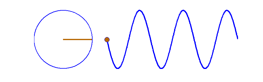
Fig.
7. A travelling sinusoidal wave. Each point along the wave executes SHM as shown by the circle. The waveform advances to
the right one wavelength in a time of one period. Matlab script: ag_sine_circle.m.
Animated gif: ag_sineC.gif
Energy transfer in a sinusoidal wave
Consider
a sinusoidal wave formed on a stretched string. The equation of a wave
travelling to the right (+X direction) is
The
total energy density u
is

And
the energy flux S
is

We
need to find the average energy flux for one complete period of the motion,
Scycle
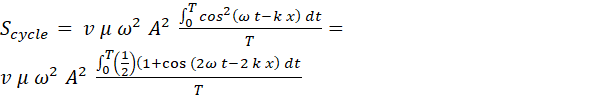
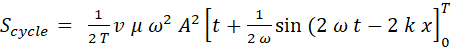
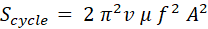
Scycle
corresponds to the average power transferred along the string by the motion
associated with the travelling sinusoidal wave. This energy transfer is
proportional to the square of the amplitude A,
the square of the frequency f and the speed of
the wave v. Remember, a wave
is a mechanism for the transfer of energy from one place to another, without
the transfer of any material. For example, tsunami waves travel across the
open ocean at speeds of hundreds of kilometres per hours and when they hit
the shoreline they have large amplitudes and we
know that the energy carried by such waves is enormous.
Video
clip Japan 2011 tsunami http://www.youtube.com/watch?v=2uJN3Z1ryck
|