[1D] SUPERPOSITION OF PLANE WAVES

Ian Cooper

Please email me any corrections, comments, suggestions or additions: matlabvisualphysics@gmail.com

DOWNLOAD DIRECTORIES FOR PYTHON CODE

emPW01.py

It turns out that any optical field (e.g. pulses or a focused beam), regardless of how

complicated, can be described by a superposition of many plane wave fields. In

this article, we develop the techniques for superimposing plane waves. We begin our analysis with a discrete sum of plane wave fields and show how to calculate the intensity in this case. We will introduce the concepts of phase velocity and group velocity. The group velocity describes the motion of interference ‘fringes’ or ‘packets’ resulting when multiple plane waves are superimposed.

We can construct arbitrary waveforms by adding together many plane waves with

different propagation directions, amplitudes, phases, frequencies and polarizations.

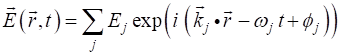
The superposition of the electric fields for plane waves expressed as a descrete sum is given by

(1)

We will consider the situation where all plane-wave components travel roughly parallel to each and assume that the vectors are real. The time-averaged intensity (irradiance) S for light composed of parallel wave vectors is then well approximated by

(2)

Note: distinction between irradiance S and intensity I . For example, 〈irradiance〉 is zero for standing waves because there is no net flow of energy, whereas equation 2 still gives a result for the intensity. Intensity specifies whether atoms locally experience an oscillating electric field without regard for whether there is a net flow of energy carried by a light field.

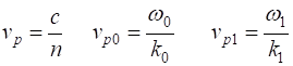
To begin our study of interference, consider just two plane waves propagating in the +Z direction with equal amplitudes given by

(3)

The phase velocities v_p (velocity of the wave crests) for the individual plane waves are

(4)

Next consider the complex (resultant) wave created from the superposition of the above

two plane waves

(5)

The two plane waves interfere, producing regions or fringes of higher and lower intensity

that move in time. Remarkably, these intensity peaks of the resultant wave can propagate at speeds quite different from either of the phase velocities of the individual waves.

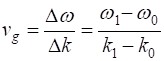
The time-averaged intensity of the complex waves travels with velocity know as the group velocity v_g

(6)

The group velocity may be thought of as the velocity for the envelope that encloses the rapid oscillations. For dispersive media, the phase and group velocities are generally different.

The Python Code emPW01.py is used to visualize the propagation of the two plane waves and the resulting complex wave. The input parameters are the number of grid points, the wavelengths (microwave wavelengths) and refractive indices.

#%% INPUTS

num = 999 # Grid points

N = 2; wL = zeros(N); n = zeros(N)

# Wavelengths wL [m]; wL[0] < wL[1]

wL[0] = 20e-3; wL[1] = 25e-3

# refractive indices n: n[0] > n[1]

# longer wavelength must have a lower value for refracticve its refractive index

n[0] = 1.1; n[1] = 1.00

#%% CALCULATIONS

c = 3e8 # speed of light

k = 2*pi/wL # propagation constant

w = c*k/n # omega: angular frequency

T = 2*pi/w[0] # period wave 1

vP = w/k # phase velocities

vG = (w[1] - w[0]) / (k[1]- k[0])

L = 20*wL[0] # Z axis range

z = linspace(0,L,num)

F = 200; t = linspace(0,20*T,F)

# Spatial electric field at time ts

ts = 0*T # ts = 0 for animation

E0z = exp(1j*k[0]*z)*exp(-1j*w[0]*ts)

E1z = exp(1j*k[1]*z)*exp(-1j*w[1]*ts)

Ez = E0z + E1z

S = 0*Ez # intensity

#%%

wp = (w[0]+w[1])/2; kp = (k[0]+k[1])/2

wg = (w[0]-w[1])/2; kg = (k[0]-k[1])/2

vG = wp/kp

The results of the calculations are displayed in the Console Window

wL0 = 0.020 m wL1 = 0.025 m

n0 = 1.100 n1 = 1.000 m

vP0 = 2.727e+08 m/s vP1 = 3.000e+08 m/s

vG = 1.636e+08 m/s

vR = 2.864e+08 m/s

A plot of the electric fields at time t_s and as an animation of the time development of the electric fields and intensity are displayed in the Figure Windows.

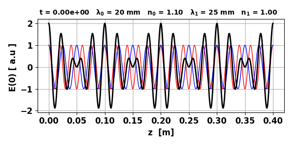
Fig. 1. Dispersive medium: electric fields at time t = 0.

Fig.2. Dispersive medium: electric fields for the two plane waves, resultant electric field, intensity, and intensity for the time-averaged over the rapid oscillations.

v_P0 = 2.727x10⁸ m/s v_P1 = 3.000x10⁸ m/s v_g = 1.636x10⁸ m/s v_R = 2.864x10⁸ m/s

The rapid oscillations in the intensity corresponds to the Poynting flux where the rapid oscillation peaks in figure 2 move with a phase velocity v_R derived from the average and average values of the two plane waves

(7)

The group velocity v_g may be thought of as the velocity for the envelope that encloses the rapid oscillations. In general, v_g and v_p are not the same. This means that as the waveform

propagates, the rapid oscillations move within the larger modulation pattern, for example, continually disappearing at the front and reappearing at the back of each modulation. The group velocity is identified with the propagation of overall waveforms.

Figures 3 and 4 shows the propagation of the plane waves in a non-dispersive medium where n₁ = n₂. In this case the phase velocities, group velocity and the velocity of the rapid fluctuations in intensities are all equal.

wL0 = 0.020 m wL1 = 0.025 m

n0 = 1.100 n1 = 1.100 m

vP0 = 2.727e+08 m/s vP1 = 2.727e+08 m/s

vG = 2.727e+08 m/s

vR = 2.727e+08 m/s

Fig. 3. Non-dispersive medium: electric fields at time t = 0.

Fig. 4. Non-dispersive medium: electric fields for the two plane waves, resultant electric field, intensity, and intensity for the time-averaged over the rapid oscillations.

v_P0 = v_P1 = v_G = v_R = 2.727x10⁸ m/s