|
COMPUTATIONAL OPTICS SUPERPOSITION OF WAVES Ian Cooper matlabvisualphysics@gmail.com DOWNLOAD DIRECTORY FOR PYTHON CODES PYTHON
CODES op002.py op002B.py op002C.py Superposition
of three waves: inputs wavelengths, amplitudes and initial phase angles SUPERPOSITION
PRINCIPLE Often a number of waves arrive at the same location at
the same time or exist together along the same direction. On most occasions
you can used the superposition principle to know the resultant wavefunction.
The superposition principle of electromagnetic waves may be expressed in
terms of vector equations
However, for the present we will consider unpolarized
light or when the field vectors are parallel and treat the electric or
magnetic field as scalar quantities. So, the resultant wavefunction due to
the superposition of N harmonic waves propagating in the z direction
is This is a valid approach, as the scalar theory applies to
each component of the electric or magnetic field, but it does not account for
all effects of very high amplitude waves, for example, the non-linear effects
of high-power laser light interacting with matter. Superposition
of waves of the same frequency The Python Code op002.py simulates the superposition of three
harmonics waves. The input variables are the wavelengths, amplitudes and
initial phase angles. #%% # Inputs:
wavelength [m], amplitude, initial phase angle [rad] >>> wL = zeros(3); wL[0] = 500e-9; wL[1] = 500e-9; wL[2] = 500e-9 A = zeros(3); A[0] = 1.2; A[1] = 0.9; A[2] = 0.5 phi = zeros(3); phi[0] = 0; phi[1] = pi/2; phi[2] = -pi/4 Amax =
2 # max
amplitude for plots Nt =
299
# number of steps Nz =
999
# Z axis grid tEnd = 4 # number
of periods for simulation for time grid zEnd = 4 # number
of wavelengths for z grid If the three harmonics waves have the same wavelength
(hence frequency) and are travelling in the same z direction, then the
resultant wave is another harmonics wave of the same frequency but with a
different amplitude and phase. #%%
COMPUTATIONS # Model
parameters c =
3e8
# speed of light in vaccum [m/s] k = 2*pi/wL
# propagation constant [rad/m] f = c/wL # frequency [Hz] w =
2*pi*f #
angular frequency
[rad/s] T =
1/f
# period
[s] tMax = tEnd*T[0]; zMax
= zEnd*wL[0] t = linspace(0,tMax,Nt) z = linspace(0,zMax,Nz) tG, zG = np.meshgrid(t,z) #
Wavefunctions: --> (-)
<-- (+) u1 = A[0]*exp(1j*(k[0]*zG - w[0]*tG + phi[0])) u2 = A[1]*exp(1j*(k[1]*zG - w[1]*tG + phi[1])) u3 = A[2]*exp(1j*(k[2]*zG - w[2]*tG + phi[2])) u = u1 +
u2 + u3
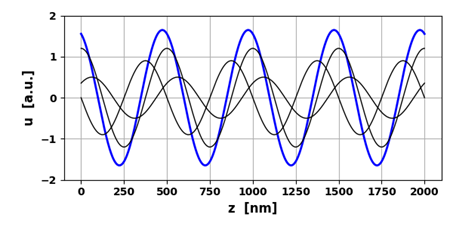
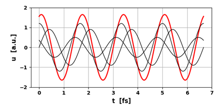
Fig. 1.
The resultant wave due to the superposition of three waves propagating
in the same direction with the same frequency is another harmonic wave of the
same frequency. op002.py
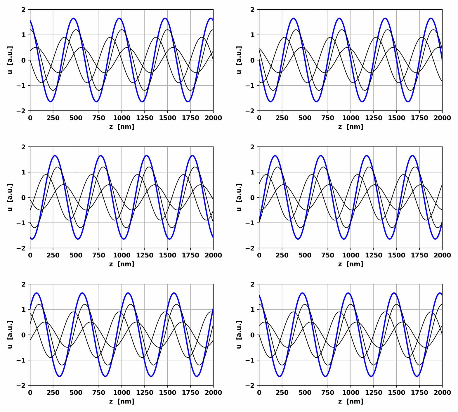
Fig
2. Animation of the three harmonic waves of the same frequency propagating in
the same direction and the resultant harmonic wave.
op002.py Random
and coherent sources It is important that one distinguishes two important
cases of superposition; ·
N coherent sources
of the same frequency, same amplitude and same initial phase. ·
N incoherent sources
of the same frequency, same amplitude and random initial phases. The resultant wavefunction of the superposition of N
waves is
Consider the instant t = 0 and z = 0 and
the amplitudes An = 1 for all N
waves, then
The intensity I of a wave is proportional to the square
of the wavefunction
For the N coherent sources, let
Icoherent = N2
|
||
|
Using
the Python code op002.py,
the summation for N incoherent sources can
be done to find the intensity by generating N random values for nR = 100 phiR = zeros(nR) uR = zeros(nR) + 1j*zeros(nR) for m in
range(nR): phiR[m]
= 2*pi*random.random() uR[m]
= exp(1j*phiR[m]) IR = np.conj(uR)*uR Itot = real(sum(IR)) print(' ') print('nR incoherent source') print('nR = %2.0f' %nR + ' Itot =
%2.2f' %Itot)
nR incoherent source
nR = 100 Itot = 100.00 We
can conclude without lots of tedious algebra that
Iincoherent = N
The
resultant intensity of N identical sources but randomly phased sources
is the sum of the individual intensities. However, resultant intensity of N
identical sources radiating in phase with each other, is N2
times the intensity of the individual sources. Inteference We
concluded that the resultant wave of the superposition of waves travelling in
the same direction with identical frequencies is another harmonic wave of the
same frequency. But are the consequences of reversing the direction of one or
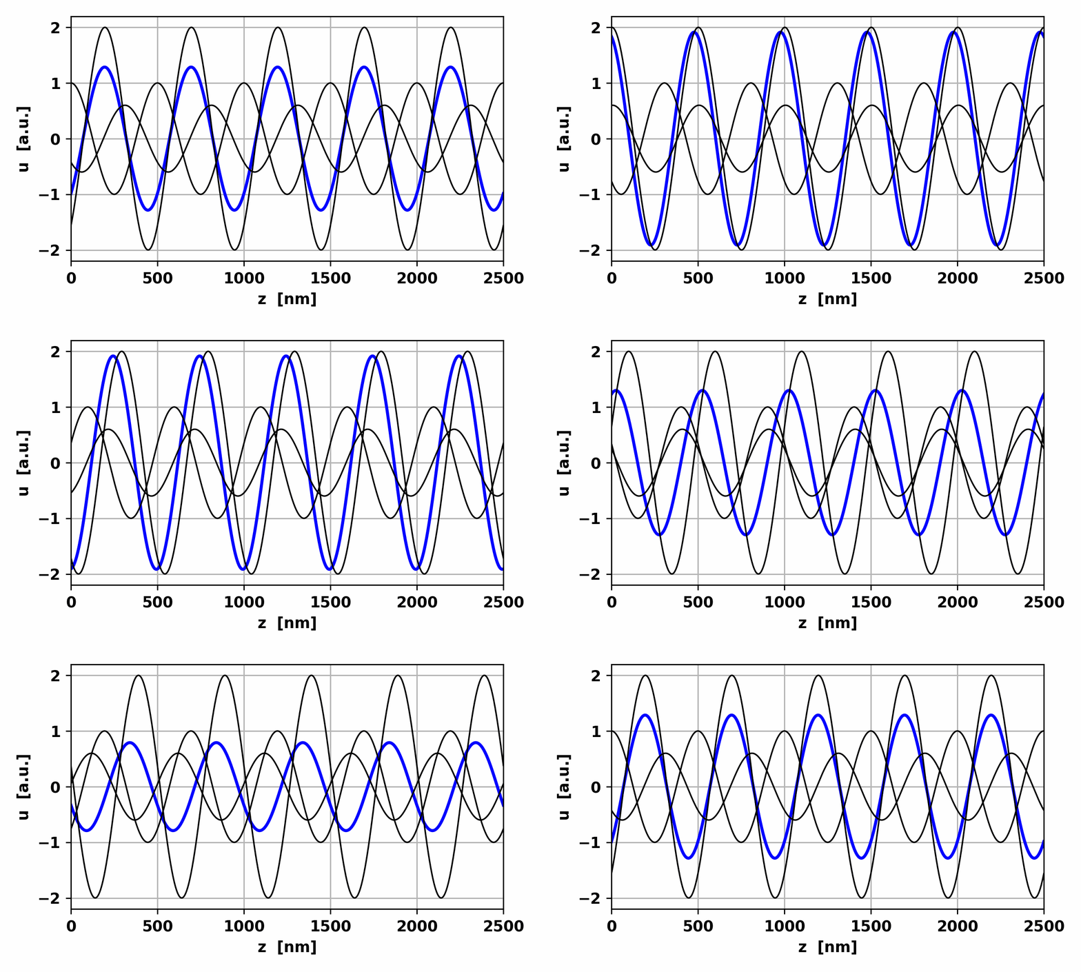
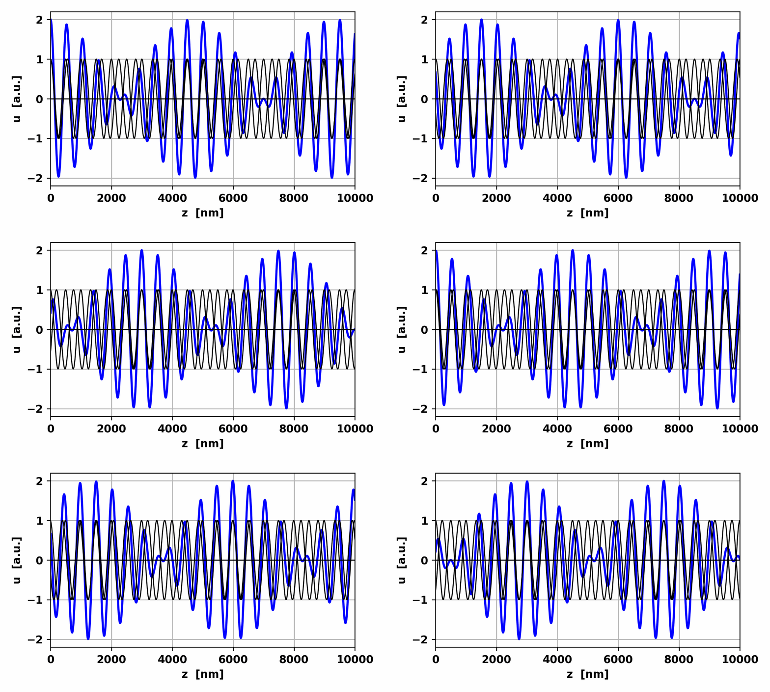
more of the waves? The Python code op002.py gives the resultant of three waves u1, u2
and u3. Figure 3 shows the animation when the direction of
the wave u2 is reversed.
Fig.
3. Waves u1 and u3 propagate in
the +z direction while wave u2 propagates in the -z direction. The resultant
wave is a harmonic wave of the same frequency but with a periodic oscillation
in its amplitude. At times the waves reinforce each other. This phenomenon is
known as constructive interference.
At other times, the waves tend to cancel each other and this is known as destructive interference. op002.py Standing
waves An
important example of interference arises when two waves with the same
frequency propagate in opposite directions. This may occur when the forward
wave experiences a reflection at some point along its path. This interference
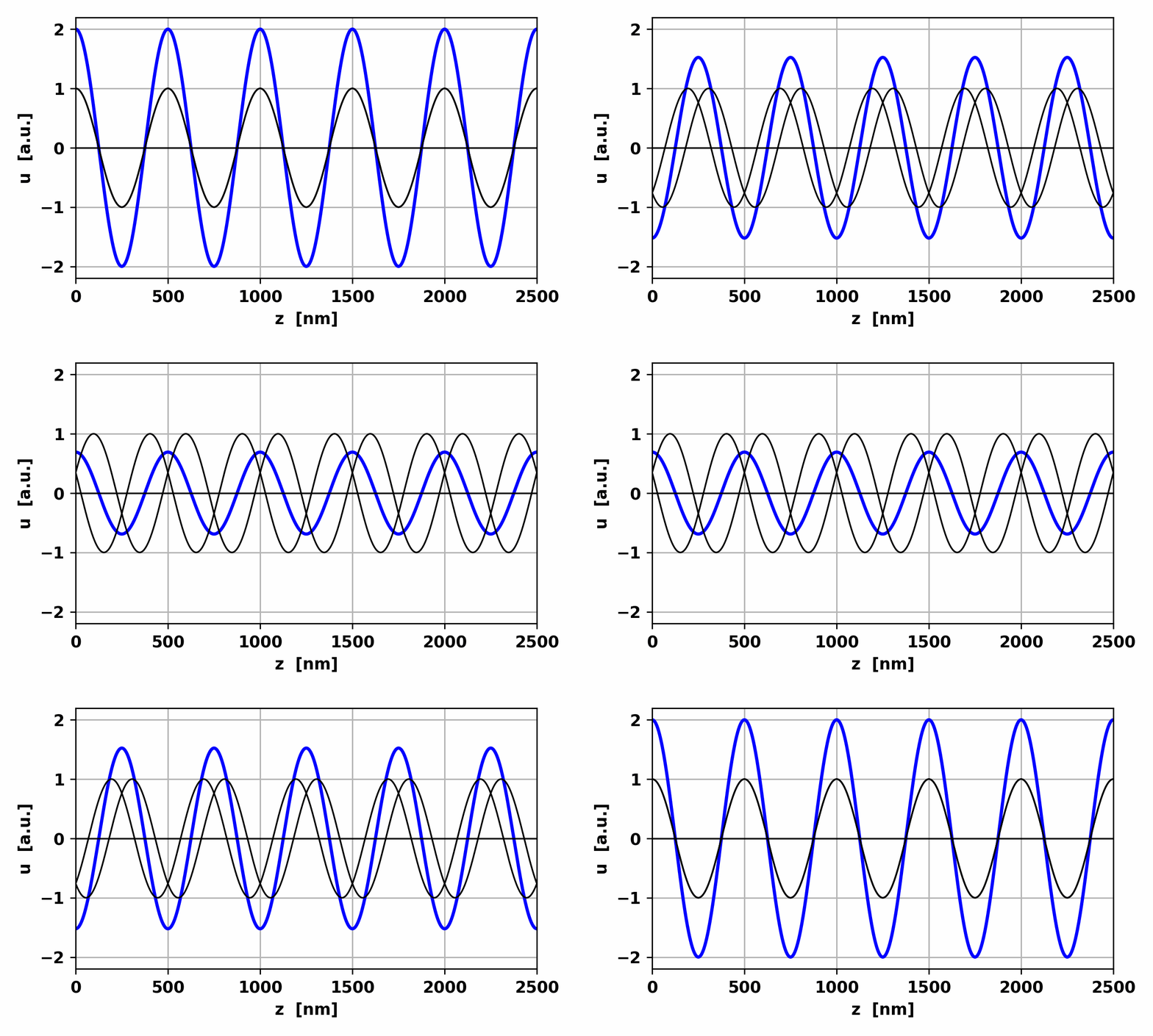
between the two waves produces a standing wave (figure
4).
Fig.
4. Standing wave due to the
interference of two waves with the same frequency and amplitude but
travelling in opposite directions. op002.py The
z locations of the nodes and antinodes are fixed, independent of time. For
the standing wave shown in figure 4, the separation between adjacent nodes or
between adjacent antinodes is Unlike
traveling waves, standing waves transmit zero energy. All the energy in the
wave goes into sustaining the oscillations between the nodes. Often
a reflected wave is reduced in amplitude as energy is absorbed during the
reflection. In this case, the two waves do not cancel exactly at the nodes
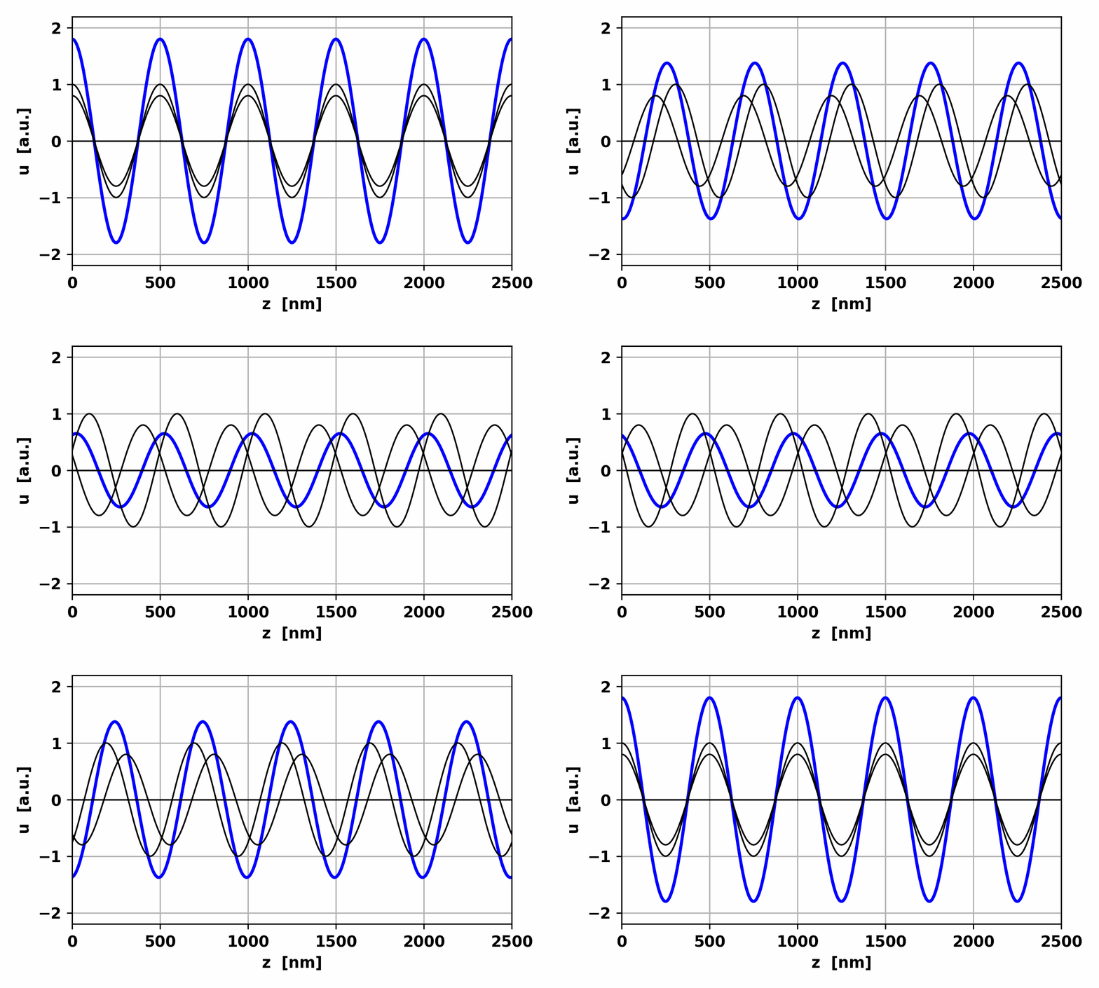
nor do they add to a maximum of 2A at the antinodes. Hence, the
resultant wave will have a traveling wave component that carries energy to
the mirror and back (figure 5).
Fig.
5. Partial standing wave. The
amplitude of the wave propagating in the -z direction is smaller than the
wave traveling in the +z direction. The positions of the nodes and antinodes
are not fixed. Observing the resultant wave carefully, you will notice the
travelling wave component. Waves
of comparable amplitude but differing in frequency The
superposition of waves with different frequencies is an important topic in
optics. Differences in frequency imply difference in wavelength and velocity.
The superposition of several such waves exhibits periodic large and small
oscillations. The
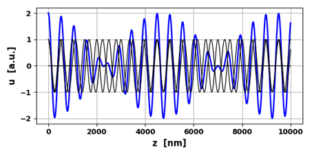
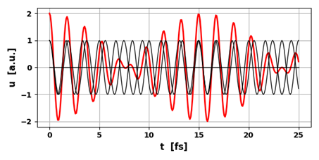
Python code op002B.py is a simulation of the phenomenon of beats where two waves of the same amplitude
but slightly different frequency combine to give the resultant wave. Beats are the periodic fluctuations in
the intensity of the wave as shown in figure 6.
Fig.
6. A beat pattern is formed when
two waves of the same amplitude but slightly different frequencies interfere
with each other.
op002B.py The
beat pattern is characterized by a sinusoidal fast oscillation and an
envelope which slowly varies sinusoidal as shown in the animation (figure 7). Fast
oscillation frequency
Slow oscillation of envelope (beat frequency) Simulation # Inputs:
wavelength [m], amplitude, initial phase angle [rad] >>> wL = zeros(3); wL[0] = 500e-9; wL[1] = 560e-9; wL[2] = 300e-9 A = zeros(3); A[0] = 1; A[1] = 1; A[2] = 0 phi = zeros(3); phi[0] = 0; phi[1] = 0; phi[2] = 0 Amax =
2.2 # max
amplitude for plots Nt =
299
# number of steps Nz =
999
# Z axis grid tEnd =
15
# number of periods for simulation for time grid zEnd =
20
# number of wavelengths for z grid Console output wL [nm] A f [Hz]
T [fs] 500
1
6.000e+14
1.667 560
1
5.357e+14
1.867 300
0
1.000e+15
1.000 f_beats [Hz] T_beats [fs]
f_fast [Hz] T_fast
[fs] 6.429e+13 15.556
5.679e+14
1.761 If
you examine the time plot in figure 6, the measured periods are: Tfast
= 1.8 fs and
Tbeat = 16
fs which
are in excellent agreement with the theoretical values
Fig.
7. Animation of the beat waveform. Non-harmonic
waves A
periodic wave which is not a harmonic wave is synthesized by the addition of
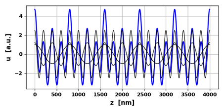
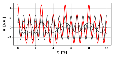
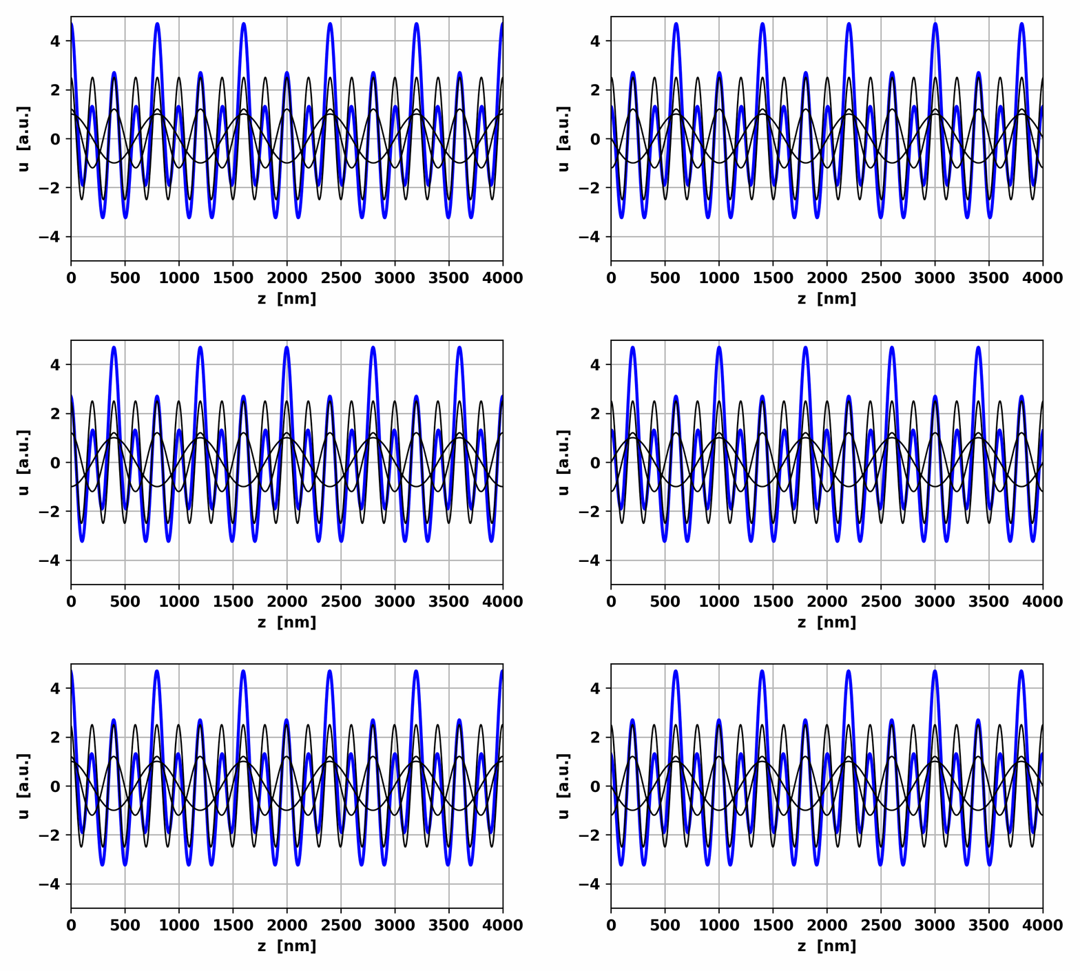
harmonic waves with different frequencies as shown in figures 8, 9 and 10. Simulation
input parameters using Python Code op002C.py wL = zeros(3); wL[0] = 200e-9; wL[1] = 400e-9; wL[2] = 800e-9 A = zeros(3); A[0] = 2.5; A[1] = 1.2; A[2] = 1 phi = zeros(3); phi[0] = 0; phi[1] = 0; phi[2] = 0 Amax =
5 # max
amplitude for plots Nt =
299
# number of steps Nz =
999
# Z axis grid tEnd =
15
# number of periods for simulation for time grid zEnd =
20
# number of wavelengths for z grid Console
output wL [nm] A f [Hz] T [fs] 200 2 1.500e+15 0.667 400 1 7.500e+14 1.333 800 1 3.750e+14 2.667
Fig.
8. Non-harmonic wave: waveform
repeats itself every 800 nm.
Fig.
9. Non-harmonic wave: waveform
repeats itself every 2.667 fs.
Fig.
10. Animation of non-harmonic
wave. |
