QUANTUM MECHANICS
TIME DEPENDENT SCHRODINGER EQUATION
FINITE DIFFERENCE TIME DEVELOPMENT METHOD SCATTERING and TUNNELLING Ian
Cooper matlabvisualphysics@gmail.com DOWNLOAD DIRECTORY FOR MATLAB SCRIPTS qm020.py (execution time ~ 60 seconds) This
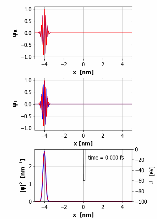
article will consider a Gaussian wavepacket representing an electron that is
scattered by a barrier represented by a potential energy function. The
wavepacket first encounters the barrier at x = 0.
The x domain
is divided into the region where x < 0
and the region where x >
0. The code qm002.py solves the
time dependent Schrodinger equation using the finite
difference time development method to produce an animation of the
scattering and/or tunnelling of the wavepacket and in the Console Window, a
summary of the probability of finding the electron in the regions x < 0
and x > 0
is displayed. If you
think about it, one can argue that almost everything we know about the
Universe is learnt as a result of scattering. Scattering
from a square barrier A
wavepacket of nominal energy <E> = E0 is scattering by a
finite square barrier of height U0 x < 0 U(x) = 0 0 < x < w U(x) = U0 x > w U(x) = 0
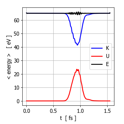
Fig.
1. Plots of the expectation energy
for the total energy <E>,
the potential energy <U> and
the kinetic energy <K> at
the end of the simulation (t = 1.54 fs). Since there are zero external
forces acting upon the system, the total energy is conserved (<E> = E0 = 65 eV,
Fig.
2. Animation of the wavepacket
encountering a finite square barrier (U0 = 60 eV
< E0 = 65 eV
and w = 0.20
nm). Probability(x<0) =
59% and Probability(x>0) =
41% It is important
to realize that the splitting of the wavefunction illustrated in figure 2
does not represent a splitting of
the electron. The splitting of the wavepacket indicates that there are two
distinct regions in which the electron can be found. In classical physics
since E0
> U0, the electron would be transmitted
across the barrier. However, quantum mechanics predicts that there is a
non-zero probability of the electron being reflected. This indeterminacy of
the location of the electron is a key characteristic feature of quantum
mechanics.
Fig.
3. Plots of the expectation energy
for the total energy <E>,
the potential energy <U> and
the kinetic energy <K> at
the end of the simulation (t = 1.54 fs). Since there are zero external
forces acting upon the system, the total energy is conserved (<E> = E0 = 65 eV, This is
an attractive potential (potential
well, U0 = -60 eV) as the
kinetic energy of the wavepacket increases on approach to the barrier. The
probability of transmission through the barrier increased from 41% to 89%
when the potential energy constant U0 changed
from +60 eV to -60 eV.
Fig.
4. Animation of the wavepacket encountering
a finite square barrier (U0 = -60 eV < E0 = 65 eV
and w = 0.20
nm). Probability(x<0) =
11% and Probability(x>0) =
89% Key
results ·
The spreading of the wavepacket
before and after the barrier is a consequence of the range of momentum values
that contribute to the wavepacket. ·
The reflection of the wavepacket by
different parts of the barrier results in interference effects within the
wavepacket. ·
The differences in behaviour between
the real and imaginary parts of the wavefunction combine to give a Gaussian
shaped probability density function ·
The reflection and transmission probabilities
are very sensitive to the parameters that specify the potential barrier. Tunnelling
of a wavepacket One of the
surprising aspects of quantum mechanics is a particle can pass through a
region that is classically forbidden. This phenonium is called quantum-mechanical tunnelling. The total expectation energy of the system
is less than the height of the barrier (U0 = 68 eV > E0 = 65
eV) in the following simulation. Classically, the electron would be reflected
and not transmitted. However, in this simulation, the quantum mechanics gives
a non-zero probability of the electron passing into the region beyond the
potential hill.
Fig.
5. The passage of the wavepacket with
<E> = E0 = 65 eV
through a finite barrier of height U0 = 68 eV
and width w = 0.20
nm. Probability(x<0) =
81% and Probability(x>0) =
19% Part of
the reason for the possible transmission of the electron through the barrier,
is that that the wavepacket has a spread of energies, some of which lie above
the top of the barrier. Even a wavepacket with all energies below the barrier
height can still tunnel through the barrier. The probability of transmission
decreases with barrier height and decreases markedly as the width of the
barrier increases. Scattering
from a finite step The
finite step potential function is represented by the potential energy
function U(x<0) =
0 U(x>0) =
U0 If the
total energy of the electron is less than step height (<E> = E0 < U0) then
the probability of it being reflected is 100%. For <E> = E0 > U0 then
the probability of transmission rapidly increases to 100% as <E>
increases above U0.
Fig.
6. The passage of the wavepacket with
<E> = E0 = 65 eV
( Probability(x<0) =
51% and Probability(x>0) =
49%
Fig.
7. The passage of the wavepacket with
<E> = E0 = 100
eV ( Probability(x<0) =
7% and Probability(x>0) =
93% |