QUANTUM MECHANICS
ANIMATIONS COMPOUND STATES IN A FINITE SQUARE
POTENTIAL WELL Ian
Cooper matlabvisualphysics@gmail.com DOWNLOAD DIRECTORY FOR PYTHON SCRIPTS qm049.py Animations: time evolution of the wavefunction and
probability density for compound states of a finite square potential well. EIGENSTATES
(STATIONARY STATES) In this article we will consider a compound
(mixed) state of the eigenfunctions for a finite square potential. It would
be easy to modify the code to examine other potential wells. The default
parameters for the well are:
grid point N = 519
eigenvalues returned M = 30 xMin = -0.20 nm xMax =
0.20 nm well width w =
0.10 nm well depth U0
= -1000 ev Physical quantities are calculated in S.I. units but results are often given in nanometres [nm]
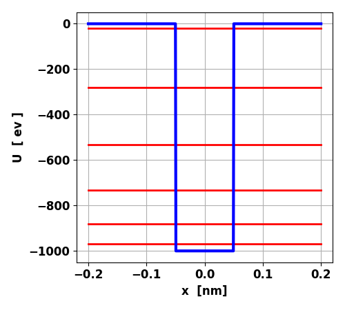
for position, electron volts [eV] for energy and attoseconds [as] for time. The potential well has six bound states and
the energy eigenvalues are: Energy
eigenvalues [ev] E1 = -970.048 E2 = -880.624 E3 = -733.192 E4 = -530.987 E5 = -281.740 E6 = -19.645
Fig. 1. Finite square well potential and
the energy spectrum for the bound states. Depth U0 = -1000, width w = 0.1 nm
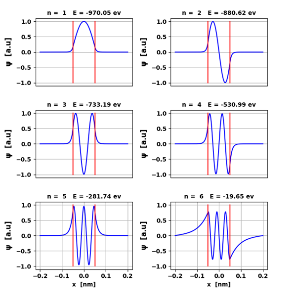
Fig. 2. The eigenfunctions
(eigenvectors) for the six bound states. The red lines
show the boundaries of the potential well.
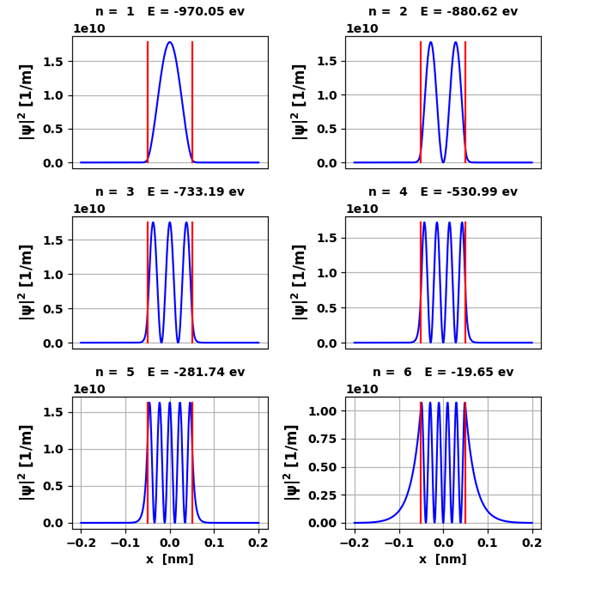
Fig. 3. The probability density
functions for the six bound states. The red lines
show the boundaries of the potential well. The eigenfunctions are normalized
for the plots so that the area under each curve is one. Note: The number of
peaks is equal to the quantum number n. The
eigenfunctions are time independent. COMPOUND
STATES: Superposition of eigenstates The wavefunction for a compound state
(mixed state) is given by
where an are a set complex numbers where
for a normalized wavefunction We can run simulations using the Code qm049.py for the summation of any two of the six
eigenstates m and n. The Code calculates expectation values for
the wavefunction and parameters describing the transition from the higher
energy eigenstate m to the lower energy eigenstate n (m
> n). In the Console Window a summary of the results is displayed.
Animations are displayed for the time evolution of the wavefunction and the
probability density. Consider a normalized compound state which is the
summation of two eigenstates m and n with wavefunction
The expectation value for the compound wavefunction can
be calculated for position and energies
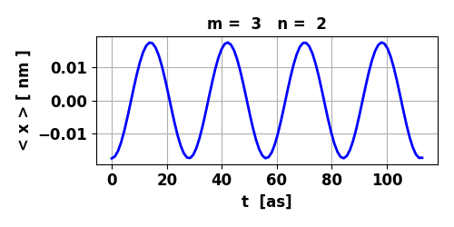
The compound states m = 3 and n = 2, m
= 3 and n =1, m = 4 and n = 1 are simulated for with the
unnormalized coefficients am = 1.00 and an
= 0.500. The normalized coefficients are am = 0.984 and an = 0.447
SIMULATIONS Compound
state m
= 3 and n = 2 Eigenstates: m = 3 n = 2 Em = -733.19
eV En = -880.62
eV Ephoton
= 147.43 eV Frequency of
emitted photon f =
3.56e+16 Hz Period of
emitted photon T =
28.05 as Wavelength of emitted photon lambda = 8.42 nm RADIATION
RATES max <x> = 1.764e-11 m electric dipole moment D = 2.826e-30 C.m rate of emission R = 2.482e-16 1/s radiative lifetime tau = 9.516e-02 s In this transition 3 à
2 a photon in the ultraviolet would be emitted with a relative short
lifetime. Energy
expectation values <U> = -971.37 eV
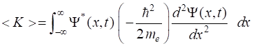
<K> = 208.69 eV
<E> = -762.68 eV The calculated expectation value for the
total energy is -763 eV. The
total energy can also be expressed as
We can interpret this result as the
probability of a measurement of the total energy made on the system is equal
to the square of the coefficient a. The result of a measurement is
either E3 = -733 eV with probability a32
= 0.8 or E2 = -880 eV with probability a22
= 0.200. The wavefunction is a superposition of two
eigenstates. Any measurement of the total energy of the system will yield an
energy eigenvalue of one of the two eigenstates. The measurement collapses
the system into the eigenstate corresponding to the eigenvalue.
Fig. 4. The expectation value for position
< x > varies sinusoidally with a relatively large amplitude.
Therefore, there is an oscillating electric dipole moment or oscillating
charge distribution. The transition from m = 3 to n = 2 leads
to the emission of a photon with energy Ephoton
= 147 eV, frequency f = 3.56x10¹⁶ Hz and wavelength
Fig. 5. Time evolution of the real (blue) and imaginary (red) parts of the wavefunction and the probability density (black).
The animation clearly shows how the charge distribution oscillates. Compound
state m
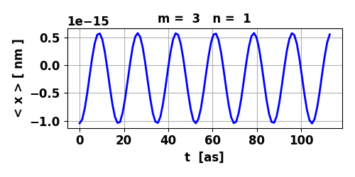
= 3 and n = 1 Eigenstates:
m = 3 n = 1 Em =
-733.19 eV En =
-970.05 eV Ephoton = 236.86 eV Frequency
of emitted photon f =
5.73e+16 Hz Period of
emitted photon T =
17.46 as Wavelength
of emitted photon lambda = 5.24 nm Energy
expectation values <U> = -965.26 eV
<K> = 200.97 eV
<E> = -780.56 eV RADIATION
RATES max <x> = -3.793e-24 m electric dipole moment D = -6.078e-43 C.m rate of emission R = 7.647e-41 1/s radiative lifetime tau = 4.963e+23 s
Fig. 6. The variation of the
expectation value of position < x > ~ 0. So, the electric dipole
moment can be considered to be zero and the transition is forbidden.
Fig. 7. The probability density changes
with time. However, since the two eigenstates have the same symmetry, no oscillating
charge distribution occurs and the transition 3 à1 is forbidden (lifetime ~ 1023
s). Compound
state m
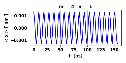
= 4 and n = 1 Eigenstates:
m = 4 n = 1 Em =
-530.99 eV En =
-970.05 eV Ephoton = 439.06 eV Frequency
of emitted photon f =
1.06e+17 Hz Period of
emitted photon T =
9.42 as Wavelength
of emitted photon lambda = 2.83 nm Energy
expectation values <U> = -946.62 eV
<K> = 327.82 eV
<E> = -618.80 eV RADIATION
RATES max <x> = 1.310e-12 m electric dipole moment D = 2.099e-31 C.m rate of emission R = 1.077e-16 1/s radiative lifetime tau = 6.530e-01 s
Fig. 8. The maximum in < x >
for the transition 4 à 1 is an order of magnitude smaller than
for the transition 3 à 2. So, the oscillations in the electric
dipole moment are about 10 times smaller. The lifetime of the transition 4 à 1 is 0.653 s while for the transition 3 à 2 is 0.095 s.
Fig. 9. The time variation in the probability
density is asymmetrical which gives rise to a small oscillating charge
distribution. The transition from m
= 4 to n = 1 leads to the emission of a photon will energy Ephoton = 439 eV, frequency f =
1.06x10¹⁷
Hz and wavelength |