QUANTUM STATISTICS
MOLECULAR DYNAMICS
MAXWELL – BOLTZMANN
DISTRIBUTION
Ian
Cooper matlabvisualphysics@gmail.com DOWNLOAD DIRECTORY FOR PYTHON CODES
PYTHON CODES SM003.py SM004.py HARD DISK MODEL SM003.py We can investigate the
Maxwell-Boltzmann distribution in Python by simulations related to molecular
dynamics by considering four hard disks of equal mass m = 1 and of
radius R =1 moving within a square of dimensions 10x10. The disks are given initial random positions (x0,
y0) and velocities (vx0, v0y).
The disks are noninteracting and
are reflected from the sides of the square (wall) and bounce off each other
in collisions. The subsequent motion of the disks can be predicted using
Newton’s laws of motion by assuming a repulsive potential between the
disk as they approach each other. However, a much simpler approach is to use
the method known as an event-driven algorithm.
The disks move with a constant velocity between collisions with either a wall
or another disk.
When a disk is within a radius of
a wall it is reflected by reversing the normal component of its velocity. def motion(x,y,vx,vy):
if x < R: vx = -vx
if x > 10-R: vx = -vx
if y < R: vy = -vy
if y > 10-R: vy = -vy
x = x + vx*dt; y = y + vy*dt
return x,y,vx,vy, The velocities of the disks after
a collision are given by the rather complex equations (https://en.wikipedia.org/wiki/Elastic_collision)
def coll(p,q): r1 = np.array([x[p],y[p]]); r2 = np.array([x[q],y[q]]) v1 = np.array([vx[p],vy[p]]); v2 = np.array([vx[q],vy[q]]) d = np.linalg.norm(r1 - r2) d2 = d**2 x1 = x[p]; x2 = x[q]; y1 =
y[p]; y2 = y[q] if d < 1*D: # V1 = zeros(2); V2 = zeros(2) z1
= v1 - 2*m2 / M * np.dot(v1-v2, r1-r2) / d2 * (r1 -
r2) z2
= v2 - 2*m1 / M * np.dot(v2-v1, r2-r1) / d2 * (r2 -
r1) v1
= z1; v2 = z2
while d < D:
x1 = x1 + z1[0]*dt; y1 = y1 + z2[1]*dt
d = sqrt((x1-x2)**2 + (y1-y2)**2)
if x1 < R: z1[0] = -z1[0]
if x1 > 10-R: z1[0] = -z1[0]
if y1 < R: z1[1] = -z1[1]
if y1 > 10-R: z1[1] = -z1[1] return v1,v2,x1,x2
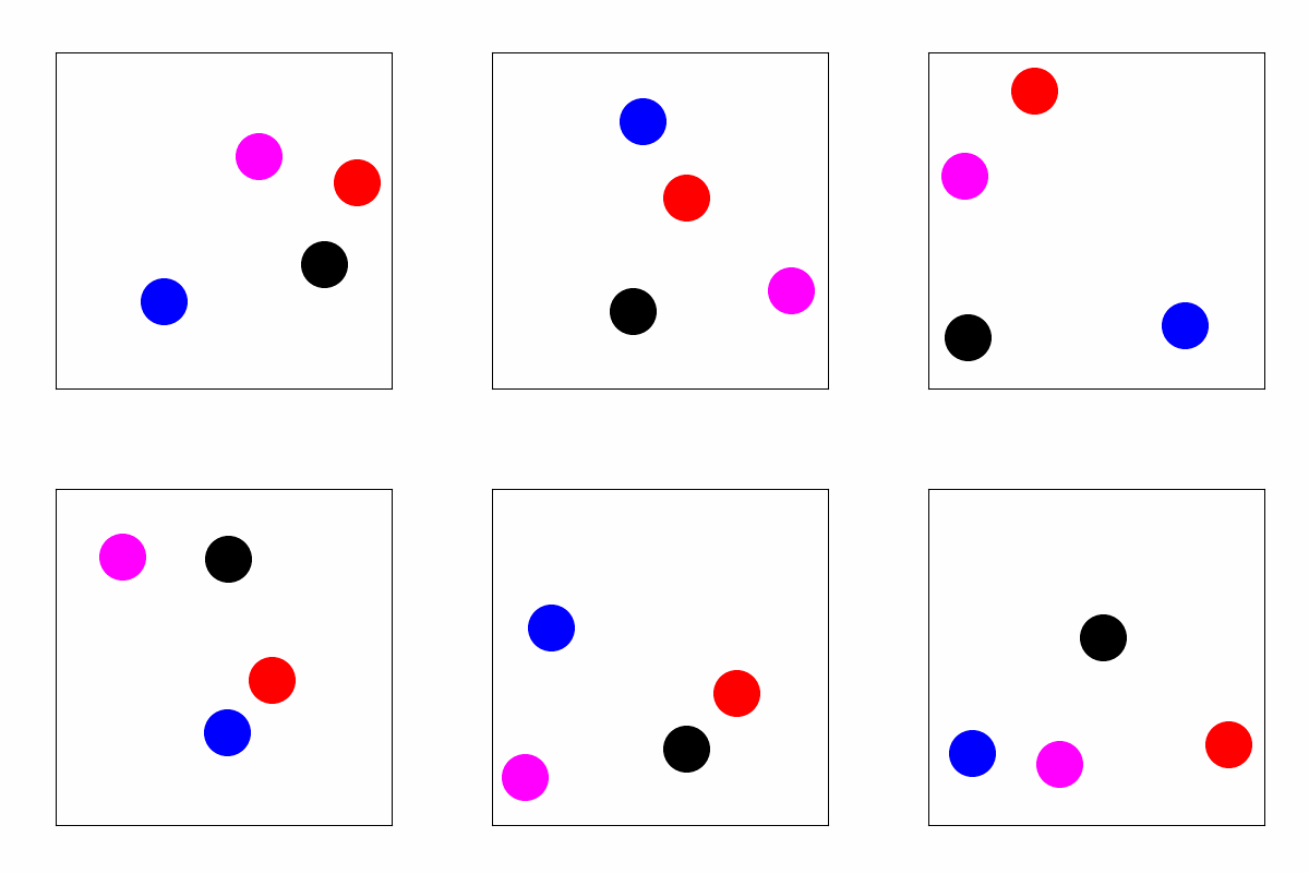
Fig. 1. Animated motion of the four hard
disks. SM003.py The random motion of the four hard disks
illustrates the motion of gas molecules inside a container. The total number
of particles and the total energy of the system is conserved. The particles
have varying speeds, some moving slowly while other move more rapidly at any
instant, but during a collision between disks, there can be an exchange of
energy between the particles which changes their velocities. An important
aspect of the simulation is that each frame shows the position of the disks
at that time and the probability of finding an arrangement of particles is
the same in each frame. GAS
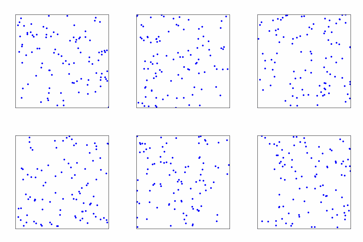
MOLECULES IN MOTION To visualize the motion of the gas
molecules, we do not need to calculate the positions or velocities. We only
need to select the positions of each gas molecule at random with the
container. Each set of positions has the same probability of occurring which
is the basis of the Maxwell-Boltzmann distribution.
Fig. 2. Animation of 100 gas
molecules. SM004.py
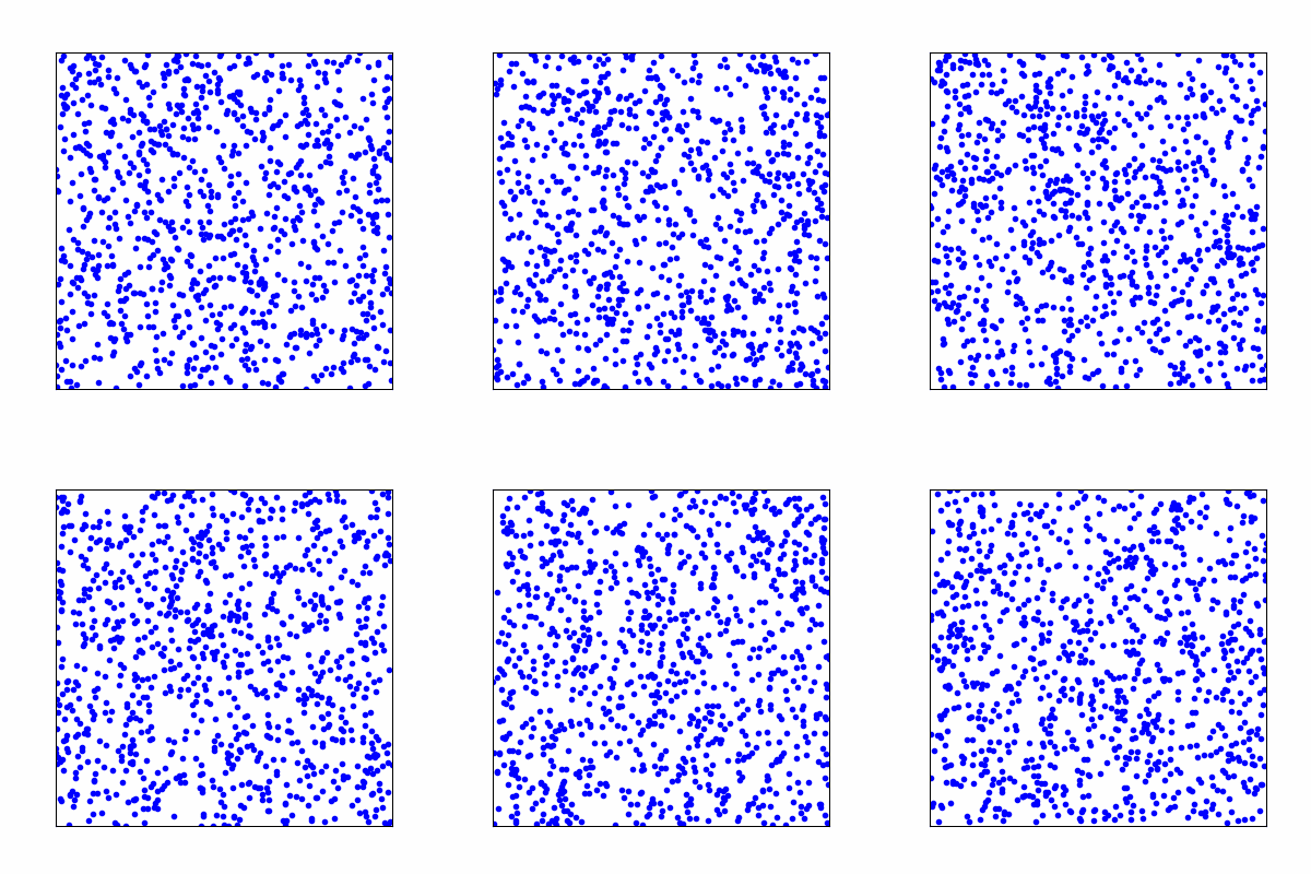
Fig 2B. Animation of 1000 gas
molecules. SM004.py |


