|
RECTLINEAR MOTION: UNIFORM ACCELERATION
Ian Cooper email
matlabvisualphysics@gmail.com
The simplest example of accelerated motion in a straight line
occurs when the acceleration is constant (uniform).
When an object falls freely due to gravity and if we ignore the effects of
air resistance to a good approximation the object falls with a constant
acceleration. A simple model to account for the starting and stopping of a
car is to assume its acceleration is uniform. Police investigators use basic
physical principles related to motion when they investigate traffic accidents
and falls. They often model the event by assuming the motion occurred with a
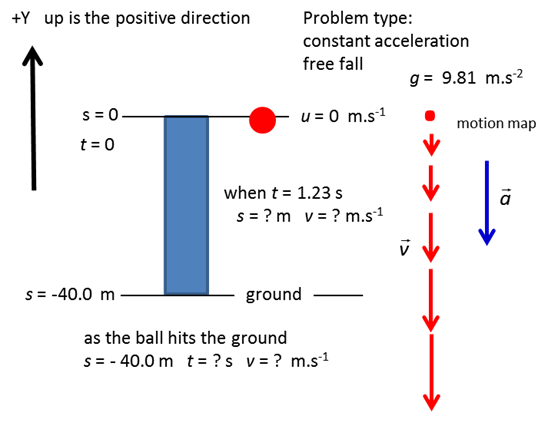
constant acceleration in a straight line To start our study of rectilinear motion with a constant
(uniform) acceleration we need a frame of reference and the object to be
represented as a particle. Since the motion is confined to the movement along
a straight line we take a coordinate axis along this line. For horizontal
motion (e.g. car travelling along a straight road) the X axis is used
and for vertical motion (free-fall motion) the Y axis is sometimes used. It
is therefore convenient to present the vector nature of the displacement,
velocity and acceleration as positive and negative numbers. We will take the
Origin of our reference frame to coincide with the initial position of the
object (this is not always done, in many books the initial location is not at
the Origin). GOTO
a Simulation - Workshop on the motion of an object moving with a constant
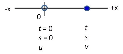
acceleration The initial state of the particle for motion along the X axis is
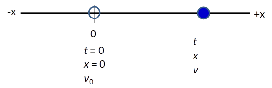
described by the parameters acceleration initial time initial displacement from origin initial velocity The final state of the particle after a time interval t is described by the parameters acceleration final time (time interval for motion) final displacement from origin final velocity
Fig. 1.
A particle at time The sign convention to give the direction for the vector nature
is summarised in the table:
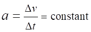
The instantaneous acceleration is defined to be the time rate of
change of the velocity and is given by equation (1) (1)
For the special case of rectilinear motion with constant
acceleration, the acceleration is (2) The
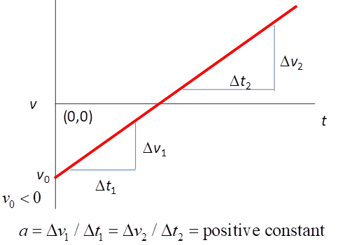
acceleration corresponds to the slope of the tangent to the velocity vs time graph. If the acceleration is constant at all
instants, then the velocity vs time graph must be a
straight
line. You know that the equation for a straight line is usually
written as For
our velocity vs time straight line graph Therefore, the straight line describing the rectilinear motion
with constant acceleration is given by equation (3) (3)
variables:
constants: The intercept at
Fig. 2.
The velocity vs time graph for the
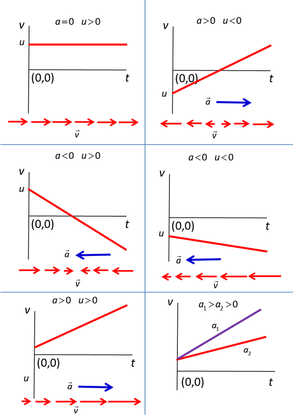
rectilinear motion of a particle with constant acceleration where Figure
(3) show six velocity vs time graphs with different
accelerations and initial velocities.
The motion of the particle is also represented by motion maps which indicate the
direction of the acceleration vector (blue arrow)
and a series of arrows representing the velocity vectors (red arrows). In answering questions on kinematics,
it is a good idea to include a motion map to help visualise the physical
situation and improve your understanding of the physics.
Fig. 3.
Velocity vs time graphs for the rectilinear
motion of a particle with different accelerations a and initial
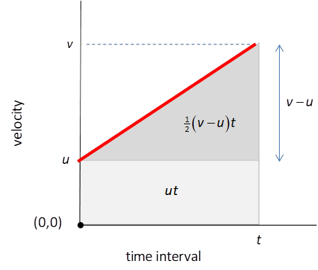
velocities The area under a velocity vs time
graph is equal to the change in displacement in that time interval. For
constant acceleration, the area under the curve is equal to the area of a
triangle plus the area of a rectangle as shown in figure (4).
Fig. 4.
The area under a velocity vs time graph is
equal to the change in displacement. For the case when the acceleration is
constant the area corresponds to the area of a rectangle plus a triangle. area
of rectangle = area
of triangle = displacement
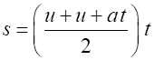
=area of rectangle + area of triangle (4) Equation
(4) can also be derived algebraically. For any kind of motion, the
displacement of the particle from the origin is given by the product of its
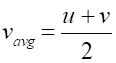
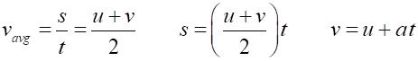
average velocity (5) For
uniform acceleration motion along a straight line, the average velocity is
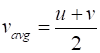
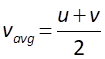
equal to the arithmetic mean of the initial and final velocities (6) Eliminating
the average velocity from these two equations results in a derivation of
equation (4) (4) Equations
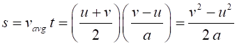
(3), (4) and (5) all contain the time interval t. We can eliminate t
from these equations to give another useful equation for uniform
acceleration. From
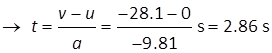
equations (3), (5) & (6) (7) The
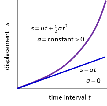
displacement s as a function of
time t which is given by equation (4) is a parabolic function involving two contributions: (1) a displacement due to the initial velocity
Fig. 5.
For the case of constant acceleration, the s vt t graph is a parabola. A
good approximation for a freely falling particle is that the acceleration is
constant. This acceleration is known as the acceleration due to gravity g. The value of g
depends upon the position of measurement – its latitude,
rocks on the Earth’s surface and distance above sea level. We will take
the value of g
to three significant figures as In this simple model, all objects irrespective of
their mass, free fall with an acceleration equal to the acceleration due to
gravity, g. Remember
that displacement, velocity and acceleration are vector quantities. The
direction of the vector along a coordinate axis is expressed as a positive or
negative number. For rectilinear kinematics problems, it is absolutely
necessary to specify a frame of reference (Coordinate axis and Origin) to
make sure that the correct sign is given to the displacement, velocity and
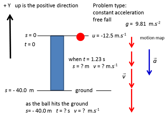
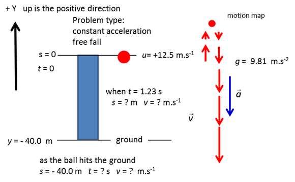
acceleration. Summary: Motion of a particle moving with a
constant acceleration
(3) (4) (7) (6) (5) s vs t graph is a
parabola slope =
velocity v vs t graph is a straight line slope = acceleration (constant) area
under graph = change in displacement a vs t graph area
under graph = change in velocity All
kinematics problems and questions can be answered using this information.
|