|
[1D] FDTD
electromagnetic wave simulations propagating in non-magnetic and uniform
dielectric media Ian Cooper Please
email any corrections, comments, suggestions or additions matlabvisualphysics@gmail.com ft_03.m Download and run the script ft_03.m. Carefully inspect the script to see how the FDTD method is implemented. Many variables can be changed throughout the script, for example, type of excitation signal, boundary conditions, time scales, properties of the media. View ELECTROMAGNETISM USING THE FDTD METHOD Simulation 1 Free Space
Propagation Nz =
400
Number of grid points for Z space flagS
= 1
Pulse zS
= 20
Source: Z location A = 1
Amplitude width = 25
Width of pulse centre
= 100
Time step for center of pulse flagBC
= 1
Absorbing boundary conditions M2 = round(Nz/2) Index
for start of Medium 2 eR1 =1 S1 = 0
Relative permittivity & conductivity Medium 1 eR2 = 1 S2 = 0
Relative permittivity
& conductivity Medium 2 Note: The absorbing
boundary conditions only apply to the case for the propagation of the wave in
free space (
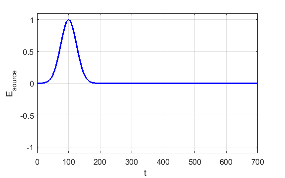
Fig.1 Gaussian source. A
“hard
source” is used because a specific value is imposed on the
FDTD grid. However, the value of Ex at the source point added to the source
gives a “soft source”. With a hard source, a propagating
pulse will see the value and be reflected, because a hard value of Ex looks
like a metal wall to FDTD. With a soft source, a propagating will just pass
straight through.
Ex(ct,zS) = source(ct)
hard source
Ex(ct,zS) = Ex(ct,Zs)
+ source(CT) soft
source
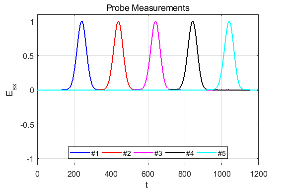
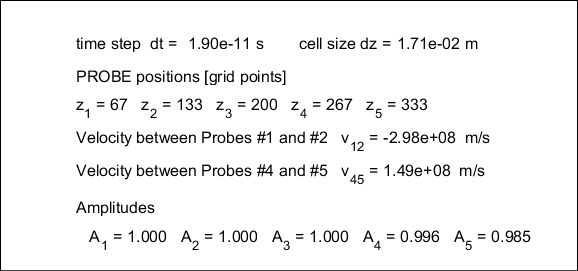
Fig. 2. The electric field at five probe
positions as functions of time. The time variation of the source electric
field near z = 0 excites an electromagnetic wave that spreads from the source
point. The wave propagates at the speed light in a vacuum c0. Time and position are not independent variables. The time step dt and the grid spacing dz are connected through the stability condition
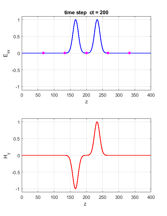
Fig. 3.
Animation of the propagation of the electromagnetic wave. The right-hand
screw rule gives the direction of propagation. The fingers of the right-hand
curl from the direction of Ex to the
direction of Hy
and then the thumb gives the direction of propagation. The energy
in an electromagnetic wave resides in the medium through which it propagates,
even in free space. The flow of energy is measured by the Poynting
vector
Fig. 4. You can vary the number of time steps to view the position of the electromagnetic wave at different times. Simulation
2 Propagation
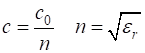
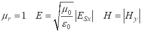
in non-magnetic and non-lossy uniform dielectric media For a
non-magnetic and non-lossy dielectric medium, the speed of propagation c
of an electromagnetic wave depends on the refraction index n
of the medium. The refractive index n is a
function of the relative permittivity
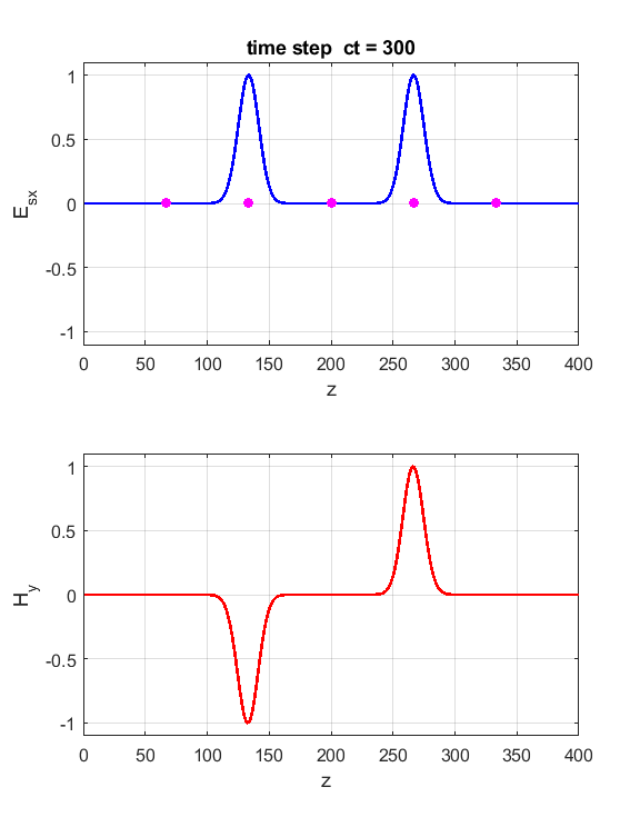
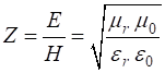
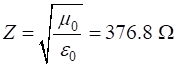
Fig. 5.
Propagation of a Gaussian pulse in a medium with relative permittivity of 4. The impedance of free space is Numerical results are displayed in Figure Window. For example, a pulse originating from the centre of Z space when eR1= 1 and eR2 = 4.
We can change the boundary conditions to set the electric field (PEC flagBC = 2) or the magnetic field (PMC flagBC = 3) to be zero at the ends of the Z space.
Fig. 6. Perfect Electric (PEC) boundary conditions. The Ex field and Hy field pulses are reflected at the ends of the Z space. The orientation of the fields is such that the direction of propagation of a pulse is given by the right-hand screw rule. As the pulses pass through each other they either interfere constructively or destructively.
Fig. 7. Perfect Magnetic (PMC) boundary conditions. The Ex field and Hy field pulses are reflected at the ends of the Z space. The orientation of the fields is such that the direction of propagation of a pulse is given by the right-hand screw rule. We can introduce two pulse sources and study the interference effects as the two pulses pass through each other. Just add the code for the second source E(ct,zS) = source(ct); E(ct,Nz-2) = source(ct);
Fig. 8. Interference effects of two pulses. Depending on the phase of the two pulses, the pulses either interfere constructively or destructively as they pass through each other. The EM wave is reflected from the hard source. Simulation 3 Propagation in
non-magnetic and lossy uniform dielectric media
Fig. 9. Propagation of sinusoidal EM wave in a lossy dielectric (eR = 0.025). |