|
[1D] FDTD
electromagnetic wave simulations with sinusoidal propagating waves in
non-magnetic and non-lossy uniform dielectric media Ian Cooper Please
email any corrections, comments, suggestions or additions matlabvisualphysics@gmail.com View ELECTROMAGNETISM USING THE FDTD METHOD ft_03.m Download and run the script ft_023m. Carefully inspect the script to see how the FDTD method is implemented. Many variables can be changed throughout the script, for example, type of excitation signal, boundary conditions, time scales, properties of the medium. Simulation 1: Sinusoidal source excitation Nz =
400
Number of grid points for Z space flagS
= 2
Sinusoidal wave zS
= 20
Source: Z location A = 1
Amplitude width = 25
Width of pulse centre
= 100
Time step for center of pulse flagBC
= 1
Absorbing boundary conditions eR1 =1 S1 = 0
Relative permittivity & conductivity Medium 1 eR2 = 1 S2 = 0
Relative permittivity
& conductivity Medium 2
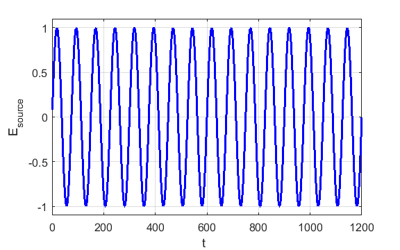
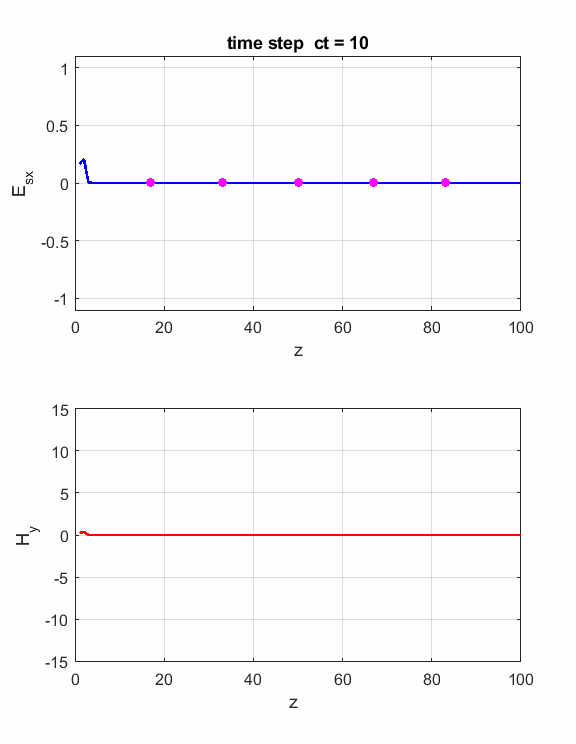
Fig. 1. Sinusoidal point source.
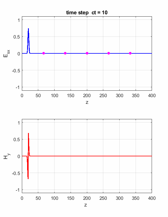
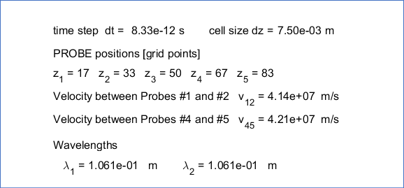
Fig. 2. A propagating sinusoidal wave in free space.
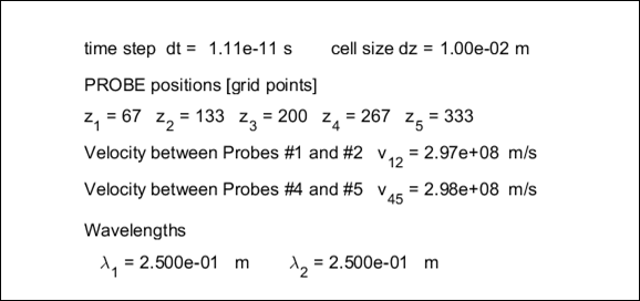
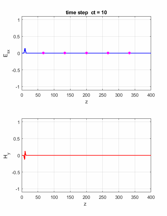
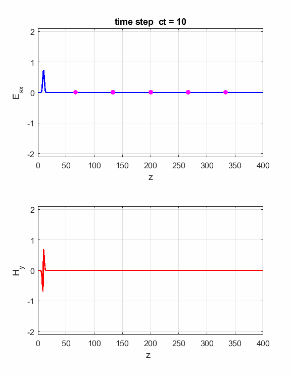
Fig. 3. Numerical results in a Figure Window The Z space grid must have enough sampling points to ensure sufficient accuracy of the results. For a sinusoidal source point, a good rule-rule-of-thumb is to have more than 10 grid per wavelength. The default settings are dz
= lambda / 25; %
cell size or grid spacing [m] dt
= dz / (sqrt(D)*c0); % time
step (time increment) [s] N.B. Depending upon the
frequency of the source, the value of dz may have to be increased or
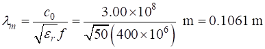
decreased to give the best plots. We can simulate an electromagnetic wave in biological tissue such as muscle. Muscle has a relative dielectric constant of about 50 at 400 MHz. So, the wavelength of the 400 MHz wave in muscle is
Fig. 3. 400 MHZ signal propagating through muscle tissue (eR1 = eR2 = 50 and dz = lambda/100). Simulation
2: A modulated
Gaussian sinusoidal pulse
We can propagate a “wave packet” which corresponds to a sinusoidal function modulated with a Gaussian envelope by setting flagS = 3.
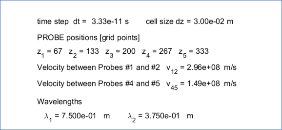
Fig. 4. The propagation of a “wave packet”. Pulse: width = 50; centre = 100; lambda = 0.75; frequency = 400 MHz.
Fig. 5. A sinusoidal EM wave striking a barrier (eR1 = 1, eR2= 4). |